Solvers: overview

Viscosity contrast

MILEVA solves Stokes flow at viscosity contrasts up to ${10}^{18}$ in the 3-D Yin-Yang shell and up to ${10}^{12}$ in the 2-D spherical annulus, measured with the code's own solvers on a viscosity step:

• 3-D, FGMRES + geometric multigrid. With geometric averaging of the viscosity at velocity faces and matrix-dependent pressure interpolation, FGMRES reaches a relative residual of ${10}^{-6}$ at every contrast from 1 to ${10}^{18}$, in 28 to 73 iterations, and needs fewer iterations as the contrast grows (43 at ${10}^6$, 28 from ${10}^{10}$ to ${10}^{18}$). Arithmetic face averaging stops converging from ${10}^8$ on.

• 2-D, sparse direct (MUMPS, UMFPACK). From contrast 1 to ${10}^9$ the solution is exact to round-off: the two independent factorisations give the same velocity to $6\times {10}^{-9}$ (mid-depth step) and $7\times {10}^{-5}$ (thin stiff lid), the divergence stays below ${10}^{-10}$ and the work-dissipation ratio $W/D$ holds its grid value to four digits. At ${10}^{12}$ the two still agree to $7\times {10}^{-6}$ (mid-depth) and $3\times {10}^{-2}$ (lid), with $W/D$ unchanged. Beyond that double precision sets the limit: a lid step still solves at ${10}^{18}$, while a stiff half-shell fails there.

Each time step MILEVA solves two kinds of linear system. The first is the coupled Stokes saddle-point system for velocity and pressure,

$$\left[\begin{array}{cc}A& G\\ B& 0\end{array}\right]\left[\begin{array}{c}\mathbf{V}\\ P\end{array}\right]=\left[\begin{array}{c}\mathbf{b}\\ 0\end{array}\right],$$

assembled as described in Discretisation. The second is the implicit temperature diffusion step. This section describes the solvers for both, how to select them, and what they cost.

Page	Contents
Direct solvers	MUMPS and UMFPACK for the 2-D Stokes system, the pressure pin, factor reuse, BiCGSTAB
Geometric multigrid	SCGS smoother, Galerkin coarse operators, BC lift, matrix-dependent pressure interpolation, FGMRES wrapper
Yin-Yang Schwarz coupling	how the two 3-D patches are solved and coupled
Parallel solvers (MPI)	one rank per patch, distributed MUMPS, block-Jacobi FGMRES, the dispatcher
Energy equation	explicit, Crank-Nicolson and backward-Euler diffusion

Which solver for which problem

Problem	Recommended	Setting	Function
2-D Stokes, any viscosity contrast	sparse direct	cfg.solverType = "mumps" or "direct"	solve_stokes_mumps, solve_stokes_v2
2-D Stokes, very large grids or solver studies	geometric multigrid	cfg.solverType = "multigrid", cfg.mgLevels ≥ 2	multigrid_stokes(::MutableGrid2D, ...)
2-D Stokes, Krylov experiments	BiCGSTAB with direct fallback	cfg.solverType = "amg"	solve_stokes_amg
3-D Stokes (Yin-Yang shell)	FGMRES + multigrid V-cycle per patch, Schwarz between patches	cfg.solverType = "multigrid", cfg.mgLevels ≥ 2	multigrid_stokes(::MutableGrid3D, ...)
3-D Stokes on several MPI ranks	dispatcher, mode = :auto	cfg.useMPI = true, launch with mpiexec	solve_stokes_distributed!
2-D temperature diffusion	Crank-Nicolson (default)	cfg.useImplicitTemp = true, cfg.implicitTheta = 0.5	diffuse_temperature
3-D temperature diffusion	explicit in the time loop	step limited by cfg.dtMax	diffuse_temperature(::Array{Float64,3}, ...)

All 2-D Stokes solvers call the same assemble_stokes(...; point_pin = true), so they solve the same discrete problem and differ only in cost and in how tightly they solve it. The 3-D branch of the time loop always calls multigrid_stokes; with cfg.mgLevels = 1 it would factorise each patch with sparse LU, whose memory outgrows a workstation at about ${10}^5$ unknowns, so keep at least two levels for every 3-D run.

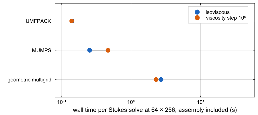
Wall time of one 2-D Stokes solve at $N_r\times N_t$ = 64 × 256 (about 49 000 unknowns), assembly included, for an isoviscous shell and for a mid-depth viscosity step of ${10}^6$. The two direct solvers take a few tenths of a second whatever the contrast; multigrid (FGMRES around a four-level V-cycle) iterated to a residual of ${10}^{-6}$ takes 2 to 3 s at this size. Script: docs/scripts/solvers_2d.jl.

Viscosity-contrast range

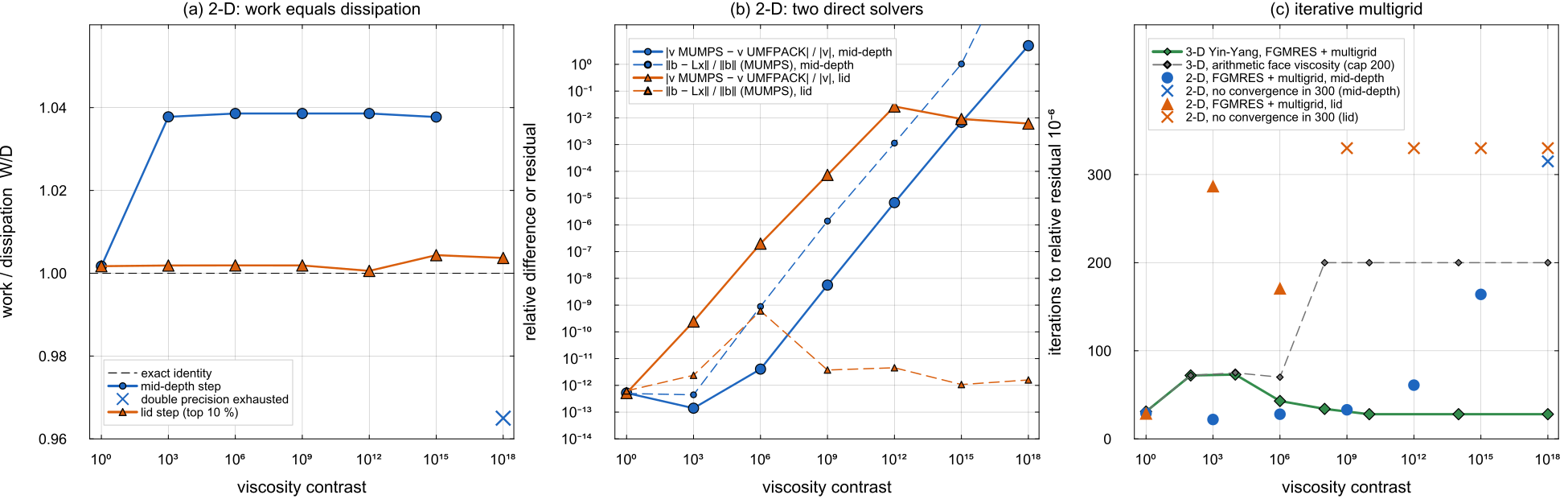
Measured by docs/scripts/solvers_contrast_range.jl. 2-D: spherical annulus $f=0.5$, $N_r\times N_t$ = 64 × 256, sinker load $100\sin (2\pi r^{\prime })\sin 2\theta$, viscosity ${10}^{20}$ Pa s below and ${10}^{20}C$ Pa s above either mid-depth or the top tenth of the shell. (a) Buoyancy work over viscous dissipation of the MUMPS solution. The identity is exact for the continuous problem; the offset of the mid-depth step is the quadrature of the dissipation across the jump and shrinks under refinement (1.084, 1.039, 1.018 at $N_r$ = 32, 64, 128, contrast ${10}^6$). (b) Relative difference between the MUMPS and UMFPACK velocities in the no-net-rotation frame (solid) and relative residual of the row-equilibrated system (dashed). (c) Iterations to a relative residual of ${10}^{-6}$: the 3-D Yin-Yang shell of the multigrid page ($N_r=N_{\theta }=12$, $N_{\phi }=36$, mid-depth step) with geometric and with arithmetic face viscosity, and the 2-D multigrid (FGMRES around a four-level V-cycle).

Measured values (2-D, MUMPS unless stated):

Contrast	$W/D$ mid-depth	$W/D$ lid	MUMPS vs UMFPACK, mid-depth	MUMPS vs UMFPACK, lid	2-D multigrid iterations (mid-depth / lid)	3-D FGMRES iterations
1	1.0017	1.0017	$5\times {10}^{-13}$	$5\times {10}^{-13}$	29 / 29	31
${10}^3$	1.0378	1.0019	$1\times {10}^{-13}$	$2\times {10}^{-10}$	22 / 287	72 (${10}^2$), 73 (${10}^4$)
${10}^6$	1.0386	1.0019	$4\times {10}^{-12}$	$2\times {10}^{-7}$	28 / 171	43
${10}^9$	1.0386	1.0019	$6\times {10}^{-9}$	$7\times {10}^{-5}$	33 / no convergence	34 (${10}^8$), 28 (${10}^{10}$)
${10}^{12}$	1.0386	1.0006	$7\times {10}^{-6}$	$3\times {10}^{-2}$	61 / no convergence	28 (${10}^{14}$)
${10}^{15}$	1.0377	1.0044	$7\times {10}^{-3}$	$9\times {10}^{-3}$	164 / no convergence	28 (${10}^{14}$)
${10}^{18}$	fails	1.0037	fails	$6\times {10}^{-3}$	no convergence	28

On the mid-depth step the 2-D multigrid matches MUMPS to $2\times {10}^{-9}$ (${10}^6$) and $7\times {10}^{-6}$ (${10}^{12}$). The thin lid, six cells deep, is coarsened below one cell on the coarse levels: there the iteration is slow at ${10}^3$, and from ${10}^6$ on it reaches the residual target with velocities that still differ from MUMPS by $7\times {10}^{-2}$. This is why the direct solvers are the 2-D choice.

Configuration fields

Field	Default	Meaning
solverType	"direct"	2-D Stokes solver: "direct" (UMFPACK), "mumps", "amg", "multigrid"
mgLevels	4	multigrid levels, including the finest; at least 2 for 3-D
mgSmooth	2	pre- and post-smoothing sweeps of the 2-D V-cycle
krylovTol	${10}^{-8}$	relative residual target of FGMRES (2-D multigrid and 3-D)
krylovMaxIter	200	FGMRES iteration cap (2-D multigrid and 3-D)
luCacheTol	${10}^{-4}$	reuse the MUMPS factor while the largest relative viscosity change stays below this
luReuseMaxIter, luReuseTol	0, ${10}^{-11}$	precondition GMRES with a stale MUMPS factor (0 disables)
useGeometricEta	true	geometric rather than arithmetic viscosity averaging at velocity faces (3-D)
useImplicitTemp, implicitTheta	true, 0.5	2-D diffusion scheme: θ = 0.5 is Crank-Nicolson, 1 is backward Euler
nTSchwarz	3	temperature Schwarz sweeps between the 3-D patches per step
useMPI, mpiNr, mpiNt	false	3-D domain decomposition (see Parallel solvers)

The nonlinear loop

With a yield law the viscosity depends on the strain rate of the flow it produces. main_SphCon.jl therefore wraps the Stokes solve in a Picard loop:

1. Solve Stokes with the current viscosity.

2. In 2-D, remove the net rotation (_net_rotation_rate).

3. Measure the relative change of $V_{\text{max}}$ from the previous sweep; stop if it is below cfg.picardTol (default ${10}^{-4}$).

4. Recompute the strain rate from the new velocity and rebuild the viscosity with composite_rheology (when cfg.useCompositeRheology is on). The new field is blended with the previous one in ${\log }_{10}\eta$ with the weight cfg.picardDamping (default 1, undamped); if the change stops decreasing, the weight is halved, down to 0.05. Damping changes the path to the fixed point, not the fixed point. Damage and viscoelastic state advance once per time step, not per sweep.

cfg.picardMax = 0 (default) means 50 sweeps when a yield law is active and one sweep otherwise; a contracting rheology without yielding needs no iteration. Steps that hit the cap unconverged are counted and logged, and every row of diagnostics.csv carries picard_n and picard_rel. With a direct solver each sweep refactorises, because the viscosity has changed.

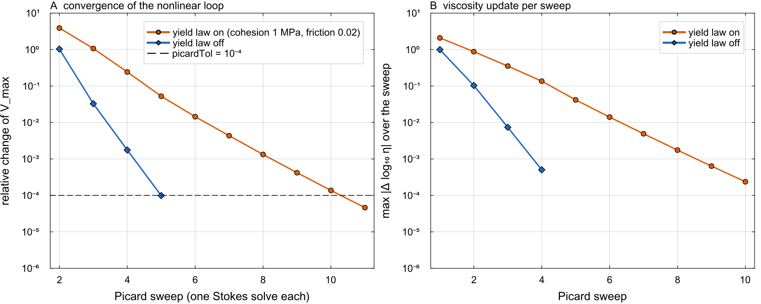
The loop above rebuilt outside the time loop from the same calls (solve_stokes_v2, _net_rotation_rate, compute_strain_rate, composite_rheology, _picard_viscosity_update), on a 64 × 256 spherical annulus with a 100 km conductive lid and a 400 K cold drip below it, started from a uniform strain rate of ${10}^{-15}$ s${}^{-1}$. (A) The stopping quantity, the relative change of $V_{\text{max}}$; (B) the largest change of ${\log }_{10}\eta$ in a sweep. With a weak yield law (cohesion 1 MPa, friction 0.02, chosen so that the lid above the drip yields; with the default 20 MPa and 0.2 nothing in this field reaches the yield stress) the loop needs 11 sweeps, with the undamped weight throughout. Without yielding the dislocation-creep nonlinearity contracts fast; the time loop solves that case once per step and starts from the previous step's strain rate. Script: docs/scripts/solvers_overview_sections.jl.

Where in the code

Topic	File	Function
Solver dispatch, Picard loop	main_SphCon.jl	time loop, step (5)
UMFPACK	solvers/solve_stokes_v2.jl	solve_stokes_v2
MUMPS	solvers/solve_stokes_mumps.jl	solve_stokes_mumps
BiCGSTAB	solvers/solve_stokes_amg.jl	solve_stokes_amg
Multigrid, Schwarz	solvers/multigrid_stokes.jl	multigrid_stokes
MPI dispatcher	solvers/solve_stokes_distributed.jl	solve_stokes_distributed!
Temperature diffusion	solvers/diffuse_temperature.jl	diffuse_temperature
Tests	tests/	test_stokes.jl, test_2d_vcycle_scgs.jl, test_mdpi_eta_contrast.jl, test_diffusion.jl, test_mpi_*.jl