Yin-Yang grid (3-D)

MILEVA's 3-D spherical shell uses the Yin-Yang overset grid of Kageyama & Sato (2004), with the coupled Stokes solve described by Tackley (2008). Two identical latitude-longitude patches, each covering a low-latitude band, are rotated against each other so that together they cover the sphere without poles. The grid is built by _setup_grid_3d in utils/setup_grid.jl; patch-to-patch interpolation lives in utils/yy_interp.jl; the coupled Stokes solve is the 3-D method of multigrid_stokes in solvers/multigrid_stokes.jl.

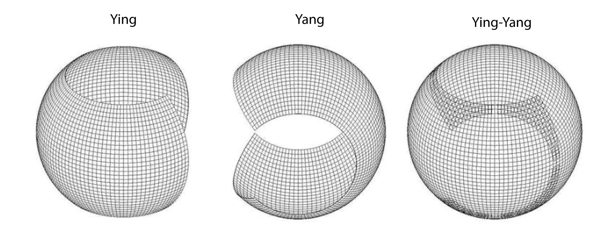
The Yin patch (left), the Yang patch (centre) and the two together (right). Both patches are the same low-latitude rectangle in their own spherical coordinates, $\theta \in [\pi /4,3\pi /4]$, $\phi \in [-3\pi /4,3\pi /4]$, i.e. 90° of colatitude by 270° of longitude. Yang is Yin turned by the Kageyama-Sato rotation below, so each patch covers the polar gaps of the other and neither has a pole. Where their edges cross, a thin band of the sphere (about 6 %) is held by both patches; this overlap is the seam across which they exchange boundary values.

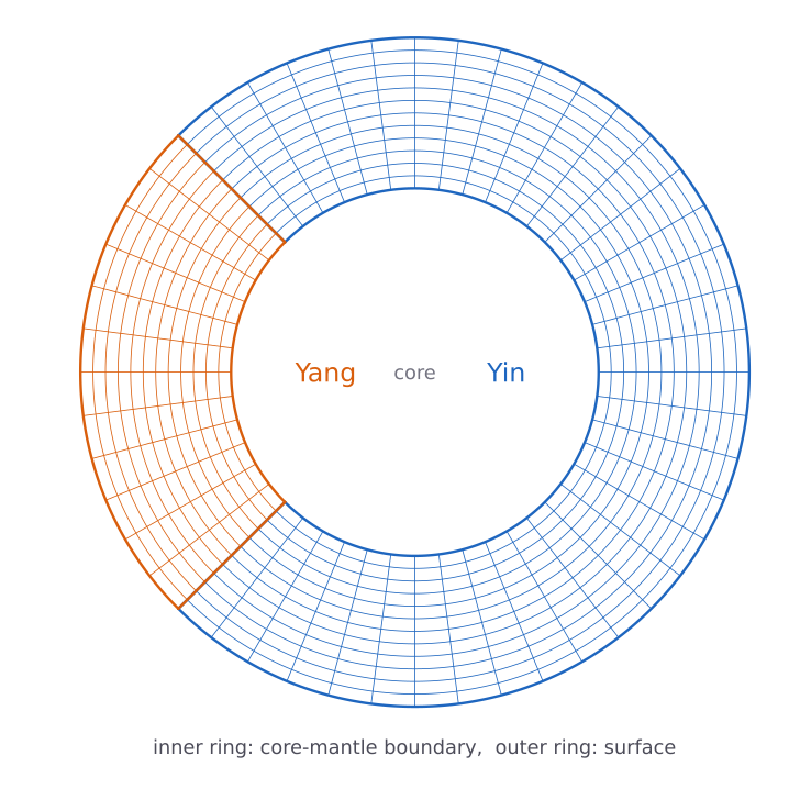
The shell in its equatorial plane. Each patch is extruded radially into $N_r$ layers between the core-mantle boundary and the surface, so the shell is $N_r$ layers of both patches. In this plane Yin supplies 270° of longitude and Yang the remaining 90°. Layers are drawn uniform here; runs usually refine them toward both walls. Every second grid line of a patch with $N_{\theta }=24$ is drawn. Script: docs/scripts/render_yinyang_cut.jl.

One patch

Each patch is a rectangle in its own spherical coordinates:

$$\theta \in [\frac{\pi }{4},\frac{3\pi }{4}],\phi \in [-\frac{3\pi }{4},\frac{3\pi }{4}],$$

90° of colatitude and 270° of longitude. cfg.Nt sets $N_{\theta }$, and $N_{\phi }=3N_{\theta }$ (rounded to a multiple of 3) gives equal angular spacing in both directions. The radial axis is the same stretched grid as in 2-D (see Discretisation). Setting cfg.chunkPhiRange below $3\pi /2$ turns the patch into a single regional chunk centred at $\phi =0$; Yin-Yang coupling then has to be off (see Grids and geometries for the chunk and the other geometries).

The grid stores one patch geometry (MutableGrid3D); the Yang patch has the same parametric grid, and its fields are held separately by the solvers.

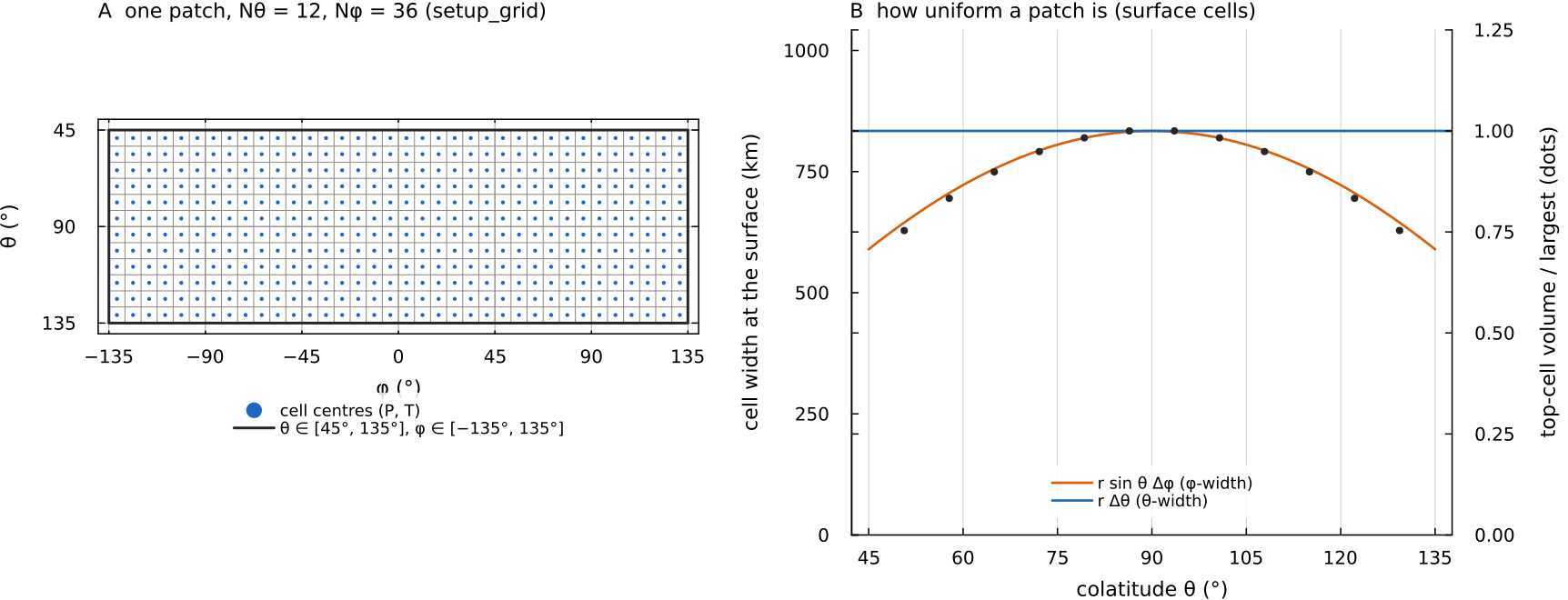
Left: the parametric grid that setup_grid builds for $N_{\theta }=12$, $N_{\phi }=36$, 7.5° in both directions, with the cell centres where pressure and temperature live. Right: the widths of the surface cells along colatitude. The $\theta$-width is constant; the $\phi$-width $r\sin \theta \mathrm{\Delta }\phi$ falls to $\sin 45°=0.71$ of its equatorial value at the patch edges, and the top-cell volumes from cell_volumes (dots) to 0.75 of the largest. A latitude-longitude grid restricted to low latitudes stays this close to uniform, which is the point of the construction. Script: docs/scripts/fig_numerics_yin_yang_sections.jl.

The Kageyama-Sato transform

Yang's Cartesian frame is Yin's frame under the rotation

$$M=\left(\begin{array}{ccc}-1& 0& 0\\ 0& 0& 1\\ 0& 1& 0\end{array}\right),(x,y,z{)}_{\text{Yang}}=M(x,y,z{)}_{\text{Yin}}=(-x,z,y),$$

which satisfies $M^2=I$, so the same map takes Yang to Yin. yy_yin_to_yang and yy_yang_to_yin in utils/setup_grid.jl implement it on $(\theta ,\phi )$ through the unit-sphere Cartesian coordinates.

Scalars ($T$, $P$) and the radial velocity $V_r$ transfer by sampling the source patch at the transformed position. The tangential components need a rotation of the local basis: at a point, Yang's $({\hat{e}}_{\theta },{\hat{e}}_{\phi })$ is Yin's rotated by an angle $\alpha$,

$${\left(\begin{array}{c}{V}_{\theta }\\ V_{\phi }\end{array}\right)}_{\text{Yang}}=\left(\begin{array}{cc}\cos \alpha & \sin \alpha \\ -\sin \alpha & \cos \alpha \end{array}\right){\left(\begin{array}{c}{V}_{\theta }\\ V_{\phi }\end{array}\right)}_{\text{Yin}},$$

returned as $(\cos \alpha ,\sin \alpha )$ by yy_rotation_yin_to_yang and yy_rotation_yang_to_yin. This is Kageyama & Sato's vector rotation (their Eqs. 22 to 24) with the opposite sign convention for the angle, used consistently in both directions; tests/test_yy_rotation_vs_ks2004.jl checks it against the paper to machine precision ($2.2\times {10}^{-16}$).

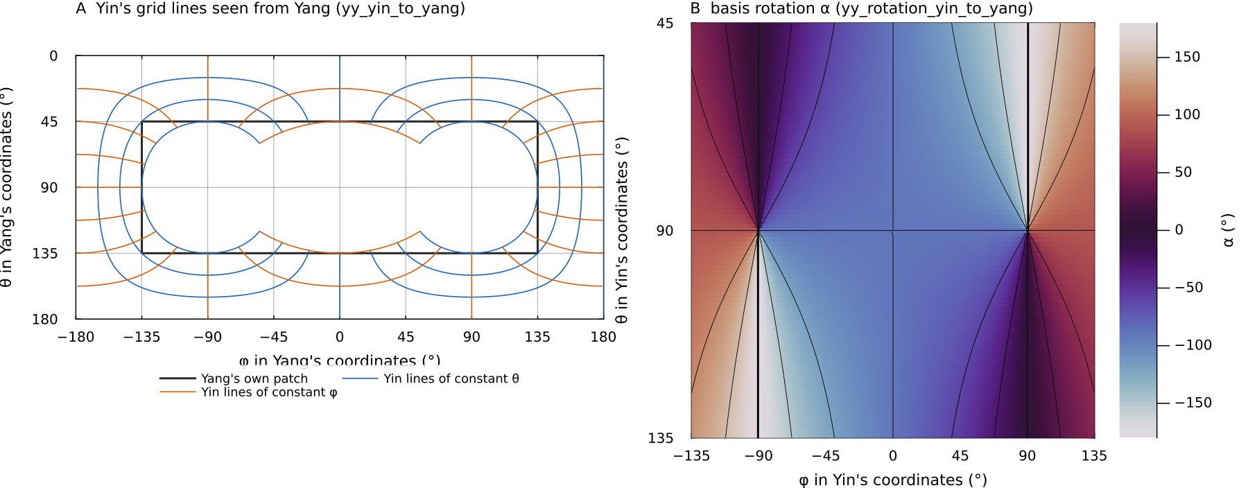
Left: lines of constant $\theta$ and $\phi$ of the Yin patch mapped into Yang's coordinates with yy_yin_to_yang. Yin covers everything outside the white "baseball" region; inside Yang's own rectangle (black), the band between that region and the rectangle is the overlap that both patches hold. Right: the angle $\alpha$ between the two local bases over Yin's patch, from yy_rotation_yin_to_yang. It winds through 360° around the two points at $\theta =90°$, $\phi =\pm 90°$, which are Yang's poles, so near them the tangential components exchange roles quickly. Mapping a position there and back returns it to $3\times {10}^{-13}$ degrees, and a vector rotated to Yang and back to $6\times {10}^{-16}$. Script: docs/scripts/fig_numerics_yin_yang_sections.jl.

Coupling the patches: Schwarz iteration

The two patches are solved separately and coupled by an overlapping Schwarz iteration on their walls. In the 3-D multigrid_stokes, each of n_schwarz rounds (default 5, fixed, no tolerance test) does:

1. yy_compute_th_bcs(:yin_dest, ...; full = true) samples Yang's current velocity at the positions that Yin's $\theta$-walls need and rotates the tangent components into Yin's basis. This gives Dirichlet values for $V_{\theta }$ on the wall faces and ghost values for $V_r$ and $V_{\phi }$ next to them.

2. The right-hand side of Yin's system is re-assembled with those values (assemble_stokes_3d(...; rhs_only = true), since the matrix does not depend on boundary values) and Yin is solved with FGMRES and a multigrid preconditioner (see Geometric multigrid).

3. The same is done for Yang from the new Yin solution.

The Schwarz residual (largest change in any velocity component over $V_{\text{max}}$) is recorded in info.schwarz_residuals. The Yin solution is returned as the primary field and Yang's in info.yang.

Interpolation is bilinear in $(\theta ,\phi )$ at each radius (_bilinear_sample_3d). A Catmull-Rom bicubic sampler (_bicubic_sample_3d) is available behind _USE_BICUBIC_YY[]; bilinear is the default.

Which walls are coupled

On the multigrid path, the one 3-D runs use, only the $\theta$-walls are Schwarz-coupled. The $\phi$-walls of each patch keep their own wall conditions. A $\phi$-wall coupling (yy_compute_ph_bcs) exists, and the single-level direct path calls it. The multigrid path leaves it out because on the equator Yin's $\phi$-wall maps onto Yang's $\theta$-wall rather than into Yang's interior. A $\delta$-cell buffer extension of the patches (cfg.δ_yy, default 0, with YYBufferTheta and YYBufferPhi in utils/yy_buffer.jl) is available and off by default.

Left: Yin's $\theta$-walls (blue) and $\phi$-walls (red, dashed) mapped into Yang's coordinates. The $\theta$-walls fall inside Yang's patch, which is what makes them suitable for Schwarz coupling; the $\phi$-walls run close to Yang's $\theta$-walls and meet them at the equator (dots). Right: the depth of each image inside Yang, measured from Yang's nearest wall. 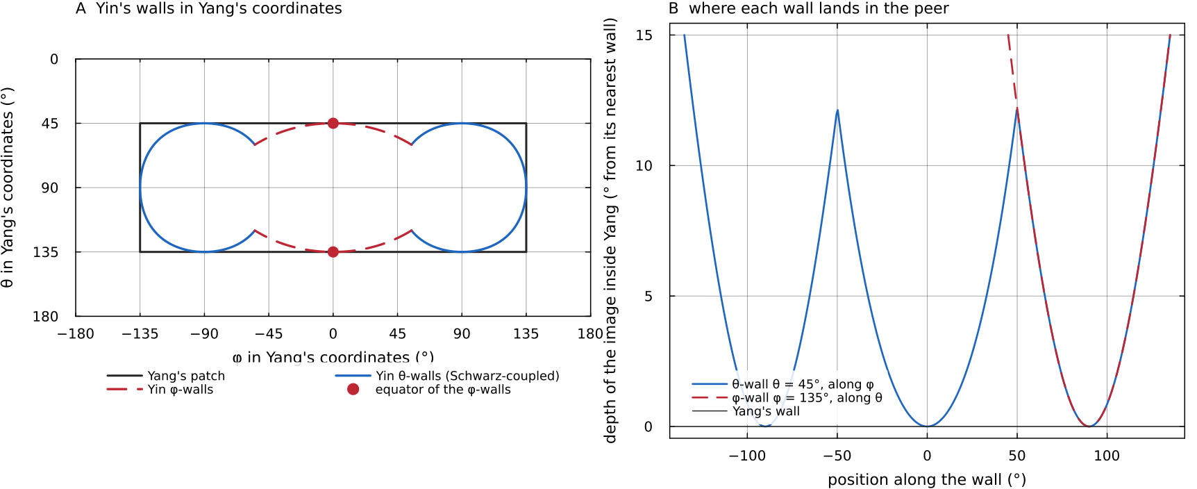Along a $\theta$-wall the image lies up to 15° inside the peer but touches its walls at three points, the corners of the overlap; along a $\phi$-wall it reaches zero exactly at the equator. Script: docs/scripts/fig_numerics_yin_yang_sections.jl.

The halo shift

Sampling the peer at the geometric ghost position does not converge: near the corners of the overlap that position maps onto, or next to, the peer's own wall, and the two walls feed back on each other. yy_compute_th_bcs therefore samples the peer a fixed angular distance past the destination wall,

$$\text{halo\_shift}=max(2,\frac{\pi /6}{\mathrm{\Delta }\theta })\text{cells},$$

that is, 30° of arc at any resolution (4 cells at $N_{\theta }$ = 12, 8 at 24, about 13 at 40), which lands the sample in the peer's interior and keeps the Schwarz residual decreasing monotonically as the grid is refined.

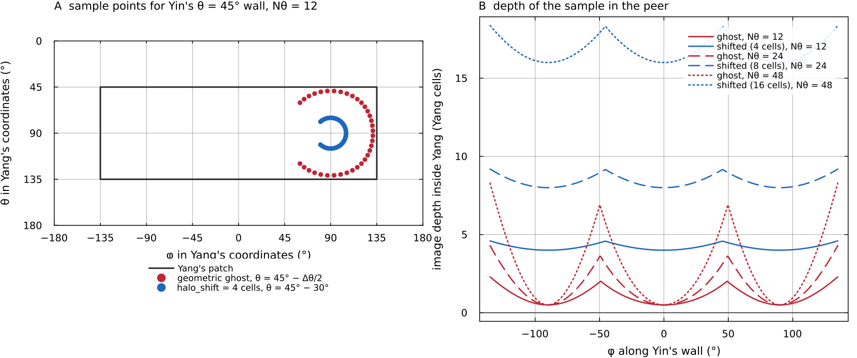
Left: in Yang's coordinates, where Yin's $\theta =45°$ wall at $N_{\theta }=12$ would sample the peer at the geometric ghost position (red) and where yy_compute_th_bcs samples it, 30° past the wall (blue). Right: the depth of each sample inside Yang, in Yang cells, along the wall for $N_{\theta }$ = 12, 24 and 48. The ghost position comes within half a cell of the peer's wall at the corners of the overlap at every resolution; the shifted sample stays at least 4, 8 and 16 cells deep, the halo shift itself. Script: docs/scripts/fig_numerics_yin_yang_sections.jl.

Seam

The shifted sample stands in for the wall value, so velocities differ slightly between the patches along the seam, more for broad flow than for localised plumes. Quantities measured across the seam are best read from refined grids.

The temperature uses the same idea with fewer steps. In the time loop, yy_compute_T_wall_bcs samples the peer temperature at each patch's $\theta$-wall faces, both patches are re-diffused with those Dirichlet values, cfg.nTSchwarz times per step (default 3), and yy_sync_T_walls! then overwrites each patch's wall-cell row with the peer value at that cell centre.

Minimum overlap

The basic Yin-Yang grid overlaps by about 6 % of the sphere. Tackley (2008, §3.1) describes a minimum-overlap grid instead, whose patch boundary follows a "baseball" curve: the corner cells that lie entirely inside the other patch are removed, so wall samples fall in the peer's interior by construction.

MILEVA offers this as an option on its rectangular patch arrays (cfg.useMinOverlapGrid, default false):

• _setup_grid_3d marks a cell as redundant when all four of its corners map into the peer's domain (live_mask, about 4.6 % of cells at $N_{\theta }$ = 12, all at the patch corners), and builds a compact live-cell index (compact_idx, live_cells).

• Redundant velocity DOFs take peer-sampled values (yy_compute_redundant_values), and their matrix columns are eliminated from the live rows so they enter as known values on the right-hand side.

• FGMRES runs on the live submatrix, with a V-cycle that also operates on the compact system.

• Markers in redundant cells are handed to the peer, and redundant-cell temperatures are taken from the peer (yy_sync_T_redundant!).

FGMRES iterations to ${10}^{-6}$ at $N_{\theta }$ = 12 for a step in viscosity of the stated contrast:

Contrast	Minimum overlap off	Minimum overlap on
$1$	40	residual $4.1\times {10}^{-3}$ after 200
${10}^6$	30	residual $6.1\times {10}^{-5}$ after 200
${10}^{10}$	13	15
${10}^{14}$	15	19
${10}^{18}$	14	15

The option narrows the seam (on an axisymmetric $Y_2^0$ load, from 19.1 % to 5.8 % at $N_{\theta }$ = 12) and converges as fast as the default at high viscosity contrast, which makes it useful for runs where seam continuity matters most.

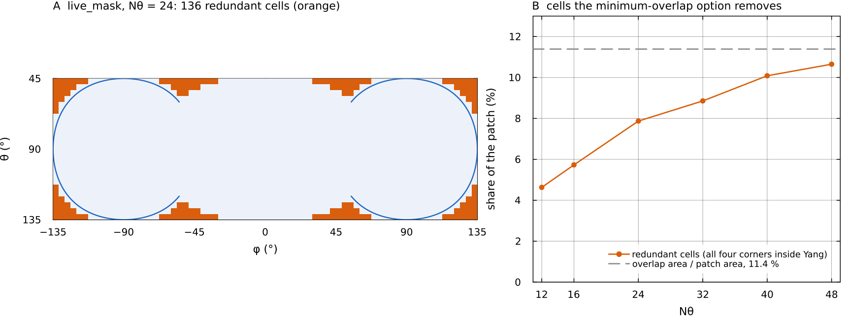
Left: the live_mask that setup_grid builds with useMinOverlapGrid = true at $N_{\theta }=24$; the 136 orange cells have all four corners inside Yang and are redundant. The blue curve is Yang's boundary seen from Yin, the baseball border the removed cells follow. Right: the redundant share of the patch against $N_{\theta }$, 4.6 % at 12 and 10.7 % at 48, approaching the area of the overlap band relative to a patch (11.4 %) as the staircase follows the curve more closely. Script: docs/scripts/fig_numerics_yin_yang_sections.jl.

Where in the code

Topic	File	Function
Patch grid, minimum-overlap mask	utils/setup_grid.jl	_setup_grid_3d, yy_yin_to_yang, yy_yang_to_yin
Vector rotation, samplers	utils/yy_interp.jl	yy_rotation_yin_to_yang, _bilinear_sample_3d, _bicubic_sample_3d
Stokes wall values	utils/yy_interp.jl	yy_compute_th_bcs, yy_compute_ph_bcs, yy_compute_redundant_values
Temperature coupling	utils/yy_interp.jl	yy_compute_T_wall_bcs, yy_sync_T_walls!, yy_sync_T_redundant!, yy_init_scalar_yang
$\delta$-buffer (off)	utils/yy_buffer.jl	YYBufferTheta, YYBufferPhi
Schwarz Stokes	solvers/multigrid_stokes.jl	multigrid_stokes(::MutableGrid3D, ...)
Two-rank MPI Schwarz	solvers/multigrid_stokes_mpi.jl, parallel/yinyang_mpi.jl	multigrid_stokes_mpi!, yy_sync_T_walls_mpi!
Tests	tests/	test_yy_rotation_vs_ks2004.jl, test_yinyang_phi_coupling_ab.jl, smoke_stokes_3d_mg.jl