Governing equations

MILEVA solves infinite-Prandtl-number thermal and thermochemical convection in a planetary mantle: a Stokes problem for velocity and pressure at every time step, coupled to an energy equation for temperature and to a marker description of composition. All fields are carried in SI units. The Stokes assembly rescales them internally before the linear solve (see Nondimensionalisation and the Rayleigh number).

This page covers the conservation equations, the two domains the code runs in, the mechanical boundary conditions and the compressibility options. The material laws and source terms that close the system have their own pages: Rheology, Buoyancy and composition, Melting and crust production, Heat sources and thermal boundaries and Free surface and isostasy.

Physical background

Why a solid mantle convects

The rock of a planetary mantle is solid on the time scale of seismic waves, yet over millions of years it creeps. At mantle temperatures, crystals deform by the slow motion of vacancies and dislocations, and a rock volume under a sustained stress strains at a rate proportional to some power of that stress. On geological time scales the mantle therefore behaves as a very viscous fluid, with a viscosity of order ${10}^{21}$ Pa s in the Earth's upper mantle as inferred from post-glacial rebound (Turcotte & Schubert 2014).

A planet loses heat through its surface while its interior is heated from below by the core and from within by the decay of radioactive isotopes. Rock that is hotter than its surroundings is less dense by $\alpha \mathrm{\Delta }T$, where $\alpha$ is the thermal expansivity, and in a gravity field it rises; colder rock sinks. Whether this motion starts, and how vigorous it becomes, depends on the competition between that buoyancy and two processes that oppose it, viscous resistance and the conduction of heat, which erases a temperature anomaly before it can move far. The ratio of the two is the Rayleigh number (below). Conduction alone is far too slow to cool a mantle. The diffusion time $D^2/\kappa$ across a 2890 km thick layer with $\kappa ={10}^{-6}$ m² s⁻¹ is about 265 Gyr, some sixty times the age of the Solar System. Convection is the process that carries the heat out, and it sets the thermal history of the interior, the stresses that act on the lithosphere and the rate at which mantle rock reaches the depths where it melts.

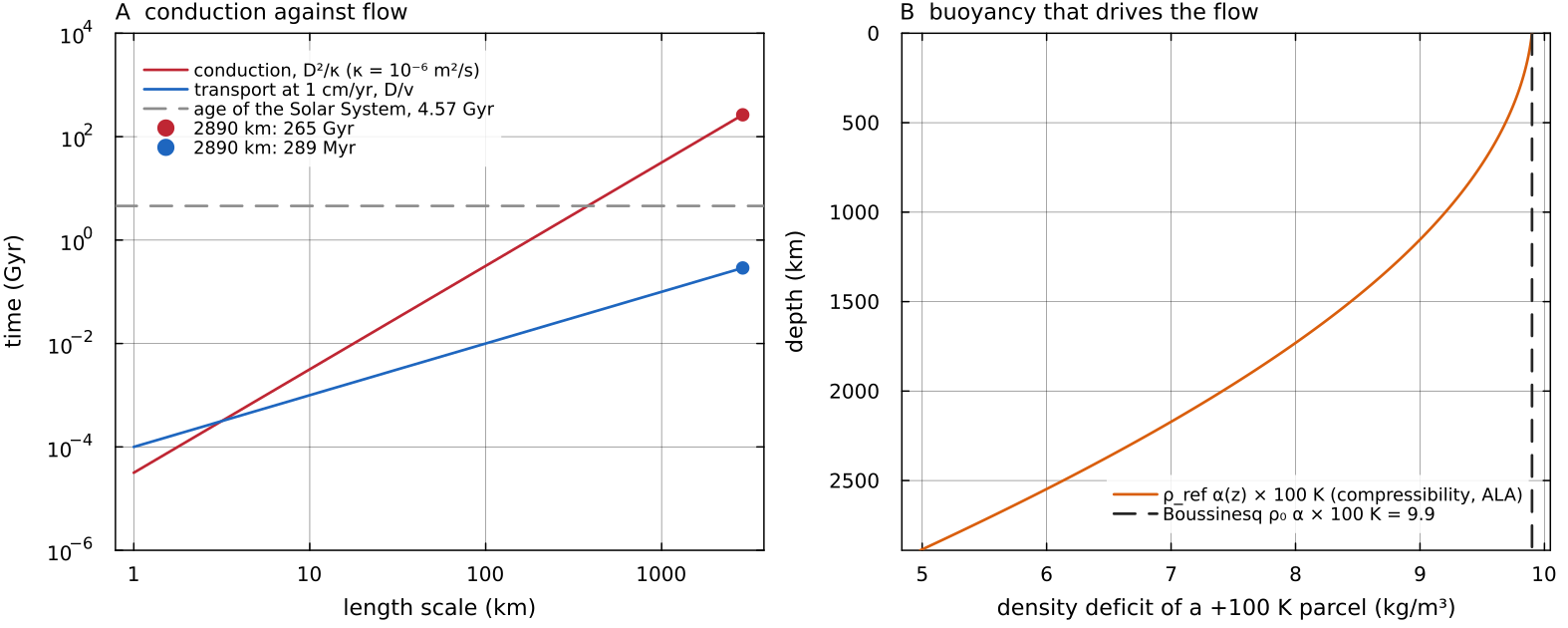
A: the conduction time $L^2/\kappa$ and the transport time $L/v$ at 1 cm/yr against the length scale. Across the 2890 km default shell conduction takes 265 Gyr and transport by flow 289 Myr. B: the density deficit of a parcel 100 K hotter than its surroundings, ${\rho }_{\text{ref}}\alpha (z)\times 100$ K from compressibility under ALA, 9.9 kg/m³ at the surface and half that at the CMB, where the expansivity is lower. Script: docs/scripts/fig_governing_equations_sections.jl.

A fluid without inertia

Mantle flow is extremely slow and extremely viscous. Two numbers make this precise. The Prandtl number $Pr=\nu /\kappa$ compares the diffusion of momentum, with kinematic viscosity $\nu =\eta /\rho$, to the diffusion of heat. The Reynolds number $Re=vD/\nu$ compares inertial to viscous forces. With $\eta ={10}^{21}$ Pa s, $\rho =3300$ kg m⁻³, $\kappa ={10}^{-6}$ m² s⁻¹, a velocity of 1 cm/yr and $D=2890$ km,

$$Pr\approx 3\times {10}^{23},Re\approx 3\times {10}^{-21}.$$

A disturbance in the velocity field is therefore damped by viscosity almost instantly compared with any thermal process, and the flow at each instant is the one that balances the forces acting at that instant. This is the infinite-Prandtl-number limit (Jarvis & McKenzie 1980; Schubert, Turcotte & Olson 2001). The momentum equation loses its time derivative and its advective acceleration and becomes the Stokes equation, a boundary-value problem with no memory of the previous velocity. All the time dependence of mantle convection then enters through the energy equation and through composition. Temperature and composition evolve, and the velocity follows them. This is why MILEVA solves a Stokes problem at every step and advances only temperature and the markers in time.

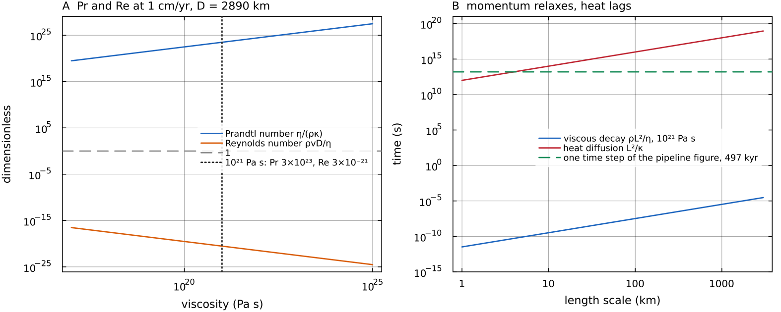
A: the Prandtl and Reynolds numbers for $\rho =3300$ kg/m³, $\kappa ={10}^{-6}$ m²/s, 1 cm/yr and $D=2890$ km, over eight orders of magnitude of viscosity. B: the time a velocity disturbance of size $L$ takes to decay by viscosity, $\rho L^2/\eta$ at ${10}^{21}$ Pa s, against the conduction time $L^2/\kappa$. Even across the whole mantle the first is a fraction of a microsecond, while one time step of the pipeline figure below lasts 497 kyr. Script: docs/scripts/fig_governing_equations_sections.jl.

The dimensionless numbers that organise the problem

Writing the equations in units of the layer thickness $D$, the diffusion time $D^2/\kappa$ and a temperature scale $\mathrm{\Delta }T$ collapses most of the material parameters into a few dimensionless groups.

number	definition	what it measures
Rayleigh number $Ra$	${\rho }_{0}g\alpha \mathrm{\Delta }T{D}^3/(\kappa \eta )$	thermal buoyancy against viscous resistance and conduction; convection needs $Ra$ above a critical value of order ${10}^3$
Péclet number $Pe$	$vD/\kappa$	heat carried by flow against heat carried by conduction
dissipation number $Di$	$\alpha gD/c_p$	strength of adiabatic heating and cooling, and of viscous dissipation, relative to the other terms of the energy equation
viscosity contrast	${\eta }_{\text{max}}/{\eta }_{\text{min}}$	how strongly temperature, pressure and composition change the viscosity; large contrasts produce a stiff surface lid
Prandtl number $Pr$	$\eta /(\rho \kappa )$	taken as infinite (see above)

Boundary-layer theory gives the leading behaviour of a vigorously convecting layer. The cold top boundary layer thickens by conduction until it becomes locally unstable, which gives a thickness of order $\delta \sim D(R{a}_{\text{cr}}/Ra{)}^{1/3}$, and the heat flow, measured by the Nusselt number $Nu$ (the convective heat flow in units of the conductive one), grows as $Nu\sim R{a}^{1/3}$ (Turcotte & Schubert 2014). Higher $Ra$ therefore means thinner boundary layers, narrower plumes and faster flow, and it is the main reason resolution requirements rise steeply with the vigour of a model.

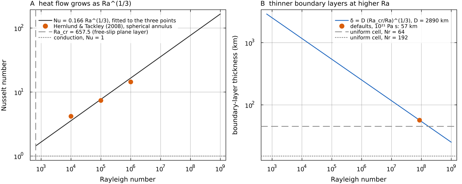
A: the scaling $Nu\propto R{a}^{1/3}$ through the isoviscous spherical-annulus values of Hernlund & Tackley (2008), Table 1, which follow it to within the scatter of three points. B: the boundary-layer thickness $\delta =D(R{a}_{\text{cr}}/Ra{)}^{1/3}$ for the 2890 km shell, with the default parameters at ${10}^{21}$ Pa s (57 km) and the uniform radial cell sizes of 64 and 192 cells for comparison. Script: docs/scripts/fig_governing_equations_sections.jl.

Typical values

With MILEVA's default parameters (SimConfig: ${\rho }_0=3300$ kg m⁻³, $g=9.81$ m s⁻², $\alpha =3\times {10}^{-5}$ K⁻¹, $\kappa ={10}^{-6}$ m² s⁻¹, an Earth-sized shell from 3481 to 6371 km; TemperatureConditions: 4000 K at the CMB and 300 K at the surface) and $\eta ={10}^{21}$ Pa s, the formulas above give

quantity	value
$Ra$	about $9\times {10}^7$
$Di$	about 0.7 with the surface expansivity, 0.2 with the CMB value ${10}^{-5}$ K⁻¹
$Pe$ at 1 cm/yr	about 900
$\delta$ from the scaling above, with $R{a}_{\text{cr}}=657.5$ (plane layer, free-slip walls)	about 60 km

These are order-of-magnitude figures, not model outputs. The full CMB-to-surface temperature difference overstates the part that drives convection, because the adiabatic increase of temperature with depth carries no buoyancy, and the effective viscosity of a real mantle varies by many orders of magnitude.

The Earth's mantle convects at velocities comparable with plate motions, a few centimetres per year, and its surface is broken into mobile plates (Turcotte & Schubert 2014). Venus has a similar size and bulk composition but no plate tectonics today. Its surface is a single lid, interpreted as a stagnant lid or one that is renewed episodically (Solomatov & Moresi 1996; Nimmo & McKenzie 1998). Solomatov & Moresi (1996) estimate the interior viscosity beneath that lid at order ${10}^{20}$ to ${10}^{21}$ Pa s. Because $Ra$ is inversely proportional to viscosity, that range alone moves the Rayleigh number of Venus by a factor of ten, which is why viscosity is usually the first parameter to vary in a Venus study.

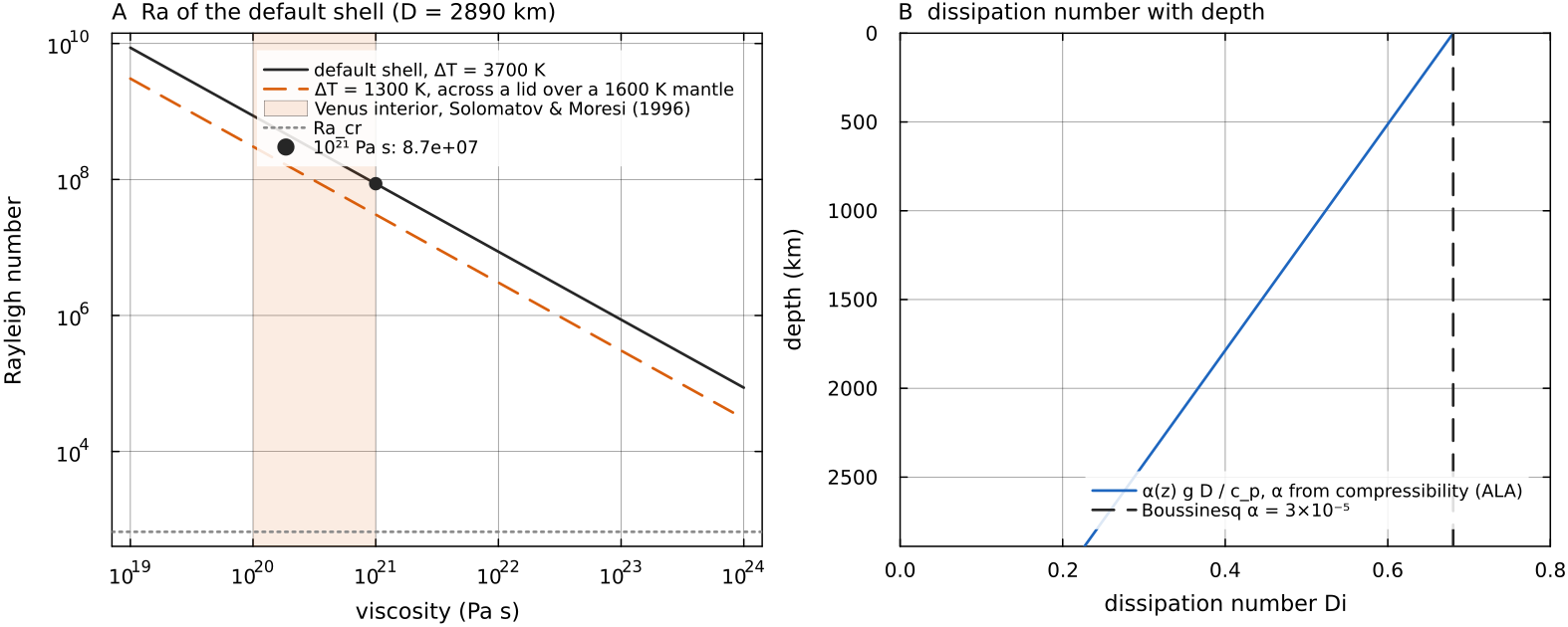
A: $Ra$ of the default shell against viscosity for the full CMB-to-surface difference of 3700 K and for 1300 K, the temperature drop across a lid over a 1600 K mantle, with the Venus interior range of Solomatov & Moresi (1996) shaded. B: the dissipation number $\alpha (z)gD/c_p$ with the depth-dependent expansivity of compressibility (ALA), 0.68 at the surface and 0.23 at the CMB, against the constant Boussinesq value. Script: docs/scripts/fig_governing_equations_sections.jl.

How one time step solves the equations

The equations are not solved all at once. Each time step goes through them in a fixed order. The temperature carried by the markers is first averaged onto the grid, and from it the code builds a viscosity and a buoyancy force. The Stokes equations then give the velocity that this force drives at this instant, because the mantle has no inertia. The velocity sets how long the step may be, the markers move with it, and finally heat is conducted, produced and consumed over that interval before the change in temperature is handed back to the markers.

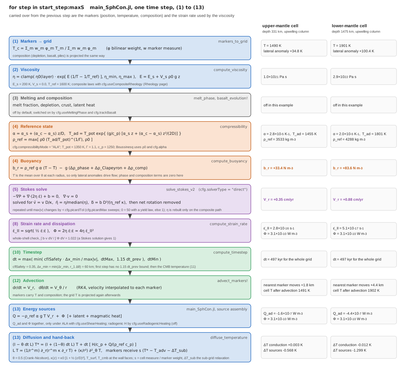
One time step of the 2-D loop in main_SphCon.jl, with its own step numbers in brackets, for the default configuration (spherical annulus, ALA, simple Arrhenius viscosity) on a 48 × 192 grid holding an adiabatic mantle with a ±100 K degree-2 temperature anomaly. The right-hand column gives the values for a cell at 331 km and a cell at 1475 km depth in the hot, upwelling column. Their anomalies of 34.8 K and 100.4 K give a buoyancy of 33.4 and 83.6 N m⁻³, an upward velocity of 0.35 and 0.88 cm/yr and a 497 kyr step, over which adiabatic cooling of the rising material lowers the temperature by 0.57 and 1.30 K while conduction changes it by less than 0.02 K. Every value is returned by the function named in its box. The script checks each against the formula shown, and the velocity and dissipation through the work-dissipation identity (1.022 over the whole shell on this grid). Script: docs/scripts/fig_governing_equations_pipeline.jl.

Momentum and mass

The momentum balance is the divergence of the full deviatoric stress against a buoyancy force $\mathbf{b}$ (positive outward, N m${}^{-3}$):

$$-\mathrm{\nabla }P+\mathrm{\nabla }\cdot (2\eta \dot{\mathit{\epsilon }})+\mathbf{b}=\mathbf{0},\dot{\mathit{\epsilon }}=\frac{1}{2}(\mathrm{\nabla }\mathbf{v}+\mathrm{\nabla }{\mathbf{v}}^{\mathsf{T}}),$$$$\mathrm{\nabla }\cdot \mathbf{v}=0.$$

That is the Boussinesq mass balance. Under ALA and TALA the 2-D annulus solves the anelastic one instead (Jarvis & McKenzie 1980), with the pressure term and the stress written to match it:

$$\mathrm{\nabla }\cdot ({\rho }_{\text{ref}}\mathbf{v})=0,-{\rho }_{\text{ref}}\mathrm{\nabla }(\frac{P}{{\rho }_{\text{ref}}})+\mathrm{\nabla }\cdot \mathit{\tau }+\mathbf{b}=\mathbf{0},\mathit{\tau }=2\eta (\dot{\mathit{\epsilon }}-\frac{1}{3}(\mathrm{\nabla }\cdot \mathbf{v})\mathbf{I}),$$

with $\mathrm{\nabla }\cdot \mathbf{v}=-V_r{\partial }_r\ln {\rho }_{\text{ref}}$ on the solution; see Compressibility modes.

Here $\mathbf{b}$ is the radial body force built by compute_buoyancy (physics/compute_buoyancy.jl) from density anomalies relative to the reference state, so the hydrostatic part never enters the solve. The thermal, phase and pile terms are lateral anomalies (the mean at each radius removed); the depletion, eclogite and crust terms are not mean-removed, and their radial mean changes only the pressure; see Buoyancy and composition. There is no inertia term and no elastic stress memory in the momentum equation.

Each term has a direct physical reading.

symbol	meaning	unit
$\mathbf{v}$	velocity of the mantle rock	m s⁻¹
$P$	dynamic pressure, the departure from the hydrostatic (reference) pressure	Pa
$\eta$	effective shear viscosity, supplied by the rheology	Pa s
$\dot{\mathit{\epsilon }}$	strain-rate tensor, the symmetric part of the velocity gradient	s⁻¹
$\mathit{\tau }=2\eta \dot{\mathit{\epsilon }}$	deviatoric (viscous) stress; under ALA/TALA $2\eta (\dot{\mathit{\epsilon }}-\frac{1}{3}\mathrm{\nabla }\cdot \mathbf{v}\mathbf{I})$	Pa
$\mathbf{b}$	buoyancy force per unit volume, positive outward	N m⁻³

The equation states that, at every point, three forces per unit volume cancel. The buoyancy $\mathbf{b}$ pushes light material up and heavy material down. The divergence of the viscous stress is the net drag that neighbouring rock exerts on a parcel that moves differently from it. The pressure gradient is the force that redistributes the flow so that no material piles up or opens a void. Because $\mathbf{b}$ contains only density anomalies relative to the reference state, the large hydrostatic pressure (about 135 GPa at the Earth's CMB; Dziewonski & Anderson

1. is not part of $P$. It is carried separately by the reference state and enters the material

laws through mantle_pressure (see Compressibility modes). The $P$ solved for is the much smaller dynamic pressure that drives and deflects the flow.

The mass equation $\mathrm{\nabla }\cdot \mathbf{v}=0$ says that a volume of rock keeps its volume as it moves. Physically rock is slightly compressible and is denser at depth; the strict mass balance of a compressible mantle is $\mathrm{\nabla }\cdot (\rho \mathbf{v})=0$. Dropping the density variation from this equation removes sound waves and pressure-volume work from the momentum problem, which is appropriate because the flow is many orders of magnitude slower than sound. The density variations that matter for driving the flow are kept in $\mathbf{b}$, and those that matter for the heat budget are kept in the energy equation under ALA. This is the logic of the Boussinesq and anelastic approximations (Schubert, Turcotte & Olson 2001; Ricard 2015). Under ALA and TALA the 2-D annulus keeps the reference density in the mass balance, $\mathrm{\nabla }\cdot ({\rho }_{\text{ref}}\mathbf{v})=0$, which still removes sound waves (only the time-independent ${\rho }_{\text{ref}}$ appears) but lets a sinking parcel be compressed as the reference state requires. This is what makes advection conserve the energy measure $c_p\int {\rho }_{\text{ref}}TdV$ of the budget.

The viscosity is what makes the problem hard. Through its strong dependence on temperature, pressure, stress and composition, $\eta$ can vary by many orders of magnitude across one model (the operator checks below go to a contrast of ${10}^8$), so the Stokes system is a linear problem whose coefficients vary enormously in space, and a nonlinear one whenever $\eta$ depends on the strain rate. The rest of this page is largely about assembling and solving that problem faithfully.

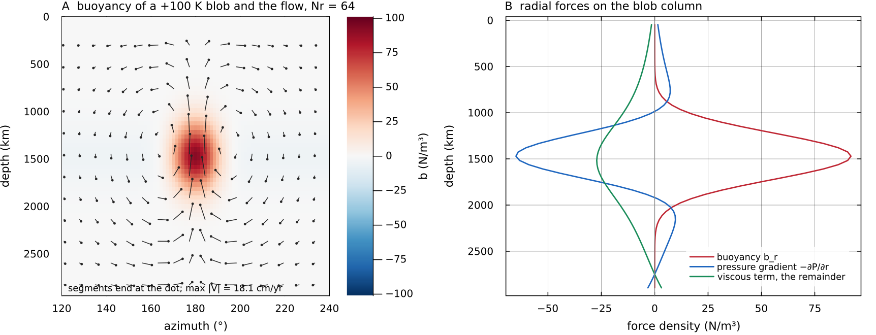
A direct solve of assemble_stokes on a Venus-sized spherical annulus (Boussinesq, $\eta ={10}^{21}$ Pa s, 64 × 256 cells, an operator illustration rather than a science grid) for a +100 K Gaussian blob at mid-depth. A: the lateral buoyancy anomaly $\mathbf{b}$ and the velocity, drawn as segments that end at the dot; the blob rises at 18 cm/yr and draws in material from the sides. B: along the column through the blob, the buoyancy, the pressure gradient and the viscous term, which is what remains; at every depth the three sum to zero. Script: docs/scripts/fig_governing_equations_sections.jl.

The 2-D operator is assembled as ∇·(2η ε̇)

assemble_stokes (solvers/stokes_assembly.jl) builds the viscous block through _viscous_block_deviatoric, which factors the operator as $L_{\text{visc}}=RS$: $S$ maps $(V_r,V_{\theta })$ to the stress $\tau =2\eta \dot{\epsilon }$ and is the only place $\eta$ appears, and $R$ is the discrete divergence of $\tau$. With the radial measure exponent $m$ (below), the strain-rate components are

$${\dot{\epsilon }}_{rr}=\frac{\partial V_r}{\partial r},{\dot{\epsilon }}_{\theta \theta }=\frac{1}{r}\frac{\partial V_{\theta }}{\partial \theta }+\frac{V_r}{r},{\dot{\epsilon }}_{\varphi \varphi }=\frac{V_r}{r}(m=2\text{only}),{\dot{\epsilon }}_{r\theta }=\frac{1}{2}[r\frac{\partial }{\partial r}(\frac{V_{\theta }}{r})+\frac{1}{r}\frac{\partial V_r}{\partial \theta }],$$

and the momentum rows are

$$\frac{1}{r^m}\frac{\partial (r^m{\tau }_{rr})}{\partial r}+\frac{1}{r}\frac{\partial {\tau }_{r\theta }}{\partial \theta }-\frac{{\tau }_{\theta \theta }}{r}-(m-1)\frac{{\tau }_{\varphi \varphi }}{r}-\frac{\partial P}{\partial r}+b_r=0,$$$$\frac{1}{r^{m+1}}\frac{\partial (r^{m+1}{\tau }_{r\theta })}{\partial r}+\frac{1}{r}\frac{\partial {\tau }_{\theta \theta }}{\partial \theta }-\frac{1}{r}\frac{\partial P}{\partial \theta }=0,$$

with continuity $\frac{1}{r^m}{\partial }_r(r^m{V}_r)+\frac{1}{r}{\partial }_{\theta }{V}_{\theta }=0$.

Under ALA and TALA three things change, all in assemble_stokes. The continuity rows carry the radial MASS flux, with ${\rho }_c$ the reference density of the cell and ${\rho }_f$ that of each radial face, both from anelastic_density:

$$\frac{1}{{\rho }_c}\frac{1}{r^m}\frac{\partial (r^m{\rho }_f{V}_r)}{\partial r}+\frac{1}{r}\frac{\partial V_{\theta }}{\partial \theta }=0.$$

The radial pressure term becomes the adjoint of those rows, $-{\rho }_f{\partial }_r(P/\rho )$, i.e. $-{\partial }_{r}P+P{\partial }_r\ln {\rho }_{\text{ref}}$, and the azimuthal one is unchanged because ${\rho }_{\text{ref}}$ does not vary along $\theta$. So the discrete gradient is the transpose of the discrete divergence in the cell-volume inner product, as in the Boussinesq case, and the pressure does no work on any velocity that satisfies the mass balance. Along an adiabatic reference ${\partial }_z\ln {\rho }_{\text{ref}}={\rho }_{\text{ref}}g/K_S$, so the extra $P{\partial }_r\ln {\rho }_{\text{ref}}$ is the buoyancy of the density change caused by the dynamic pressure, the term of the anelastic liquid approximation of Jarvis & McKenzie (1980). Finally the stress is the compressible deviator: inside $S$ each normal stress loses $\frac{2}{3}\eta \mathrm{tr}\dot{\epsilon }$, with the trace ${\dot{\epsilon }}_{rr}+{\dot{\epsilon }}_{\theta \theta }+(m-1){\dot{\epsilon }}_{\varphi \varphi }$ built from the same discrete strains,

$${\tau }_{ii}=2\eta ({\dot{\epsilon }}_{ii}-\frac{1}{3}\mathrm{tr}\dot{\mathit{\epsilon }}),{\tau }_{r\theta }=2\eta {\dot{\epsilon }}_{r\theta },$$

so $L_{\text{visc}}=RS$ is the divergence of a stress whose work is $2\eta (\dot{\epsilon }:\dot{\epsilon }-\frac{1}{3}(\mathrm{tr}\dot{\epsilon }{)}^2)\ge 0$. In the cylinder the out-of-plane ${\tau }_{zz}=-\frac{2}{3}\eta \mathrm{tr}\dot{\epsilon }$ exists but has no divergence in the plane. Rigid rotation has $\dot{\mathit{\epsilon }}=0$ and carries no mass flux, so it remains an exact null mode. Under ALA compute_strain_rate returns the deviatoric invariant and components, so the rheology, the dissipation $4\eta {\dot{\epsilon }}_{II}^2$ and the stress output see the strain rate the operator uses. The out-of-plane hoop strain ${\dot{\epsilon }}_{\varphi \varphi }=V_r/r$ exists only in the spherical annulus, where the out-of-plane direction is a latitude; the same term enters the second invariant in compute_strain_rate (utils/compute_strain_rate.jl), so the rheology sees the strain rate the operator implements.

The switch is cfg.useDeviatoricStress (default true). Setting it false assembles $\eta {\mathrm{\nabla }}^2\mathbf{v}$, which omits $2(\mathrm{\nabla }\eta )\cdot \dot{\epsilon }$ and so matches the full operator only at constant viscosity. The work-dissipation identity below is the check that exercises the viscosity-gradient term.

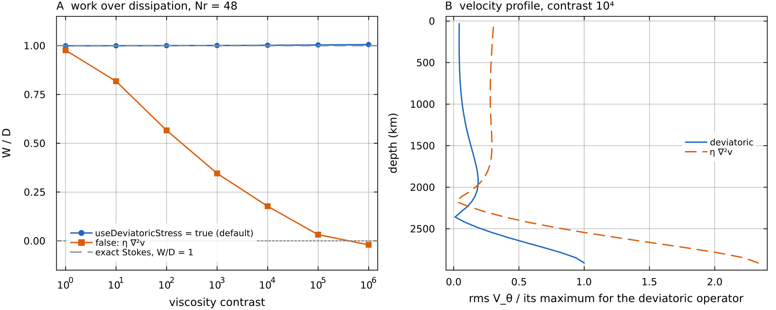
Buoyancy work over viscous dissipation for a smooth load on an exponential radial viscosity ramp, 48 × 192 cells, spherical annulus, solved with useDeviatoricStress = true and false. A: the deviatoric operator stays at $W/D=1.000$ to $1.006$ from contrast 1 to ${10}^6$; $\eta {\mathrm{\nabla }}^2\mathbf{v}$ gives 0.977 even at constant viscosity in this geometry and falls to $-0.02$ at ${10}^6$, which no Stokes solution can produce. B: the two velocity profiles at contrast ${10}^4$ differ in shape as well as in size. Script: docs/scripts/fig_governing_equations_sections.jl.

Staggered grid

The 2-D unknowns sit on a staggered (MAC) grid: $V_r$ on the $N_r+1$ radial faces, $V_{\theta }$ on the azimuthal faces and $P$ at the $N_r\times N_t$ cell centres, periodic in $\theta$. The normal stresses ${\tau }_{rr}$, ${\tau }_{\theta \theta }$ and ${\tau }_{\varphi \varphi }$ use the cell-centre viscosity, and the shear stress ${\tau }_{r\theta }$, which lives at cell corners, uses the arithmetic mean of the four surrounding cells. The 3-D assembly (solvers/stokes_assembly_3d.jl) uses the same staggering on each Yin-Yang patch and geometric means for face and edge viscosities by default (cfg.useGeometricEta = true).

The staggered arrangement goes back to Harlow & Welch (1965) and is the standard finite-difference discretisation of incompressible viscous flow in geodynamics (Gerya 2019). Placing each velocity component on the faces it crosses makes the discrete divergence of a cell a simple balance of the fluxes through its own faces, so mass conservation is exact cell by cell, and it couples neighbouring pressures directly, so the spurious chequerboard pressure mode that a collocated grid admits does not arise.

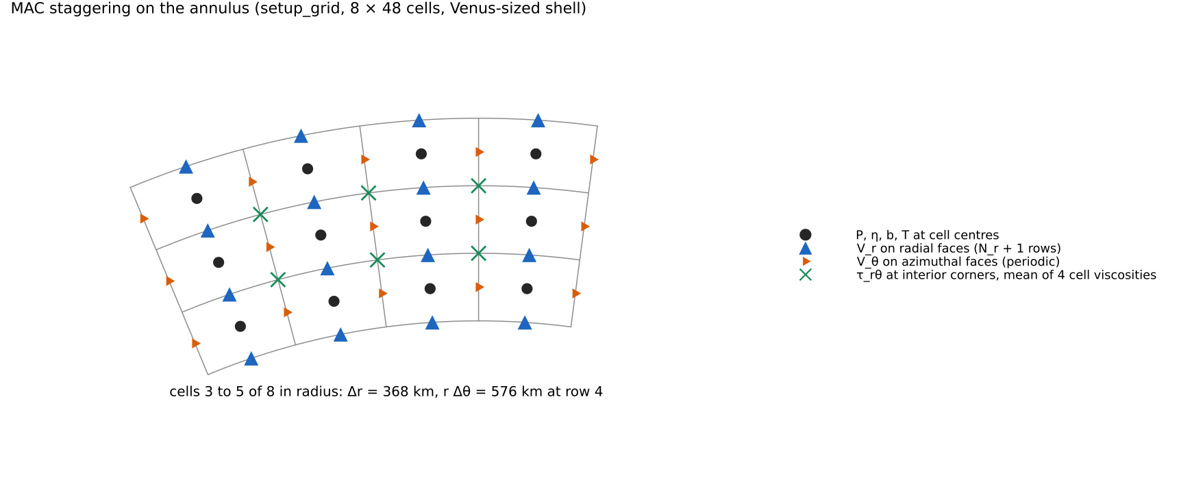
Where the 2-D unknowns live, drawn from the coordinates of setup_grid on a coarse 8 × 48 Venus-sized annulus (grid.r, grid.rF, grid.th): pressure and the cell fields at the centres, $V_r$ on the radial faces including the two walls, $V_{\theta }$ on the azimuthal faces, and the shear stress at the cell corners, where its viscosity is the mean of the four cells that meet there. Script: docs/scripts/fig_governing_equations_sections.jl.

Domains: the spherical annulus and the 3-D shell

MILEVA runs in two domains. The 2-D mesh is a full $2\pi$ annulus of $N_r$ radial by $N_t$ azimuthal cells between cfg.R_in and cfg.R_out; the 3-D mesh is a Yin-Yang spherical shell of two identical patches of $N_r\times N_{\theta }\times N_{\varphi }$ cells.

In 2-D everything that distinguishes one radially symmetric geometry from another reduces to the exponent $m$ in the shell area $A(r)\propto r^m$, returned by geometry_exponent(cfg) in utils/geometry.jl. The mesh is identical; only the metric factors change.

	2-D spherical annulus	2-D cylindrical annulus	3-D Yin-Yang shell
cfg.geometry / cfg.dim	"spherical_annulus", dim = 2 (default)	"cylindrical_annulus", dim = 2	dim = 3
measure $m$	2	1	true sphere
cell measure	$\frac{1}{3}(r_{F,\text{hi}}^3-r_{F,\text{lo}}^3)\mathrm{\Delta }\theta$	$\frac{1}{2}(r_{F,\text{hi}}^2-r_{F,\text{lo}}^2)\mathrm{\Delta }\theta$	$r^2\sin \theta \mathrm{\Delta }r\mathrm{\Delta }\theta \mathrm{\Delta }\varphi$
radial divergence	$r^{-2}{\partial }_r(r^{2}f)$	$r^{-1}{\partial }_r(rf)$	$r^{-2}{\partial }_r(r^{2}f)$
inner/outer area ratio (Venus, 3110/6052 km)	0.264	0.514	0.264

The spherical annulus is the equatorial slice of a spherical shell with the latitude-variation terms dropped. Its boundary area ratio, volume weighting and radial divergence match the sphere, which is why it is the default and the geometry every example and benchmark in this documentation uses. The cylindrical annulus over-weights the core-mantle boundary by a factor 1.95 on a Venus-sized body; it is available for comparison with cylindrical models. validate!(cfg) refuses the bare string "annulus" because the two choices give different answers.

Helpers in utils/geometry.jl (shell_measure, cell_measure, radial_flux_weight, geometry_area_ratio) give every operator the same metric: the Stokes assembly, the conservative temperature diffusion (solvers/diffuse_temperature.jl), the strain rate, the Nusselt baseline (conductive_baseline_C in physics/compressibility.jl), the core heat capacity and CMB area (physics/cmb_heat_flux.jl) and the marker weights.

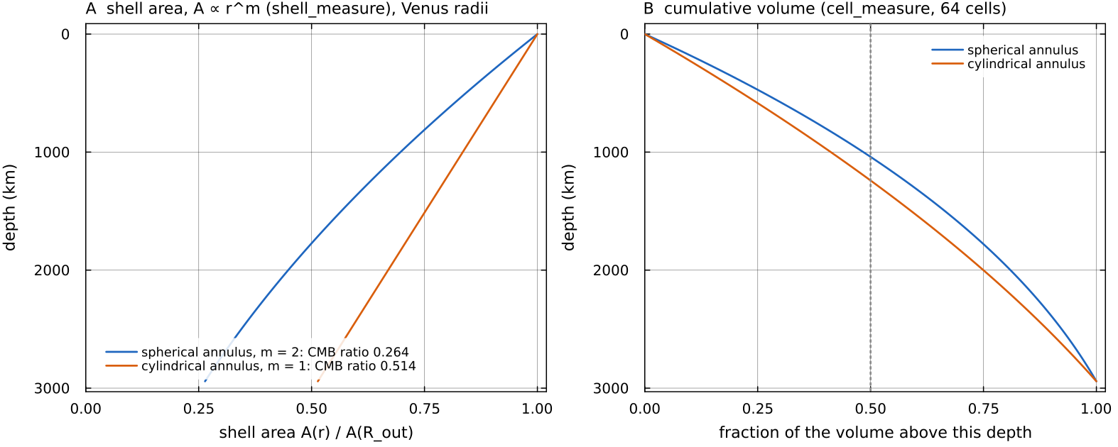
The two 2-D geometries on Venus radii (3110 to 6052 km). A: the shell area from shell_measure, with the CMB-to-surface ratios of geometry_area_ratio, 0.264 spherical and 0.514 cylindrical. B: the fraction of the volume lying above each depth, summed from cell_measure over 64 cells. Half of the spherical annulus lies above 1011 km depth, against 1195 km for the cylinder, which gives the deep mantle more weight. Script: docs/scripts/fig_governing_equations_sections.jl.

Mechanical boundary conditions and null modes

Both walls are impermeable and free slip:

wall	condition	implementation
CMB $r=R_{\text{in}}$ and surface $r=R_{\text{out}}$	$V_r=0$	identity rows on the first and last $V_r$ faces in assemble_stokes
same	zero shear traction, ${\tau }_{r\theta }=0$	the wall shear flux is dropped in _viscous_block_deviatoric
azimuth (2-D)	periodic	jminus / jplus wrap-around
3-D patch edges	Schwarz coupling to the other Yin-Yang patch	multigrid_stokes (solvers/multigrid_stokes.jl)

The top is therefore a fixed, flat surface. Deflections of it are handled separately and approximately; see Free surface and isostasy.

The 2-D system has two null modes. The pressure constant is fixed by replacing the continuity row of one central cell with a pressure pin (a single-point pin, point_pin = true, in every 2-D solver), and solid-body rotation by pinning one $V_{\theta }$ value. After every solve, with cfg.removeNetRotation = true (default), the 2-D driver then removes the rigid rotation $\omega r$ from $V_{\theta }$ with $\omega =\sum r{V}_{\theta }A/\sum r^{2}A$ (_net_rotation_rate in main_SphCon.jl), so surface velocity and lid mobility are reported in a no-net-rotation frame.

Here $A$ is the exact cell measure of the geometry, $(r_{F,i+1}^{m+1}-r_{F,i}^{m+1})\mathrm{\Delta }\theta /(m+1)$ (cell_measure), so the sums are the angular momentum and the moment of inertia in the measure $r^{m}drd\theta$; for the spherical annulus the moment of inertia is $\int r^{4}drd\theta$. Until 2026-10-14 the Boussinesq form used the cylindrical $r\mathrm{\Delta }r\mathrm{\Delta }\theta$ in both geometries, which removes a planted rigid rotation equally well but leaves a spherical-annulus frame with non-zero angular momentum whenever $V_{\theta }$ varies with depth. In 3-D the projection is not applied at all, and validate! warns once when removeNetRotation is set for dim = 3.

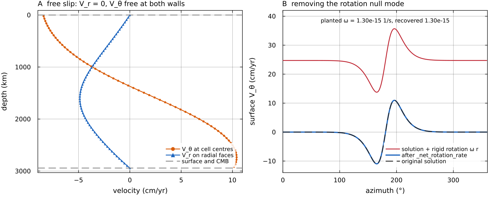
The blob solution of the momentum figure (64 × 256 cells). A: at a column 25° from the blob, $V_r$ vanishes on both walls while $V_{\theta }$ is free there, as zero shear traction allows. B: a rigid rotation $\omega r$ with $\omega =1.30\times {10}^{-15}$ s⁻¹ added to the solution and removed again by _net_rotation_rate, which recovers it and returns the original surface velocity. Script: docs/scripts/fig_governing_equations_sections.jl.

Energy equation

Temperature obeys

$$\frac{\partial T}{\partial t}+\mathbf{v}\cdot \mathrm{\nabla }T=\frac{1}{r^m}\frac{\partial }{\partial r}(r^m\kappa (r)\frac{\partial T}{\partial r})+\frac{\kappa (r)}{r^2}\frac{{\partial }^{2}T}{\partial {\theta }^2}+\frac{H_{\text{mass}}}{c_p}+\frac{Q}{{\rho }_{\text{ref}}(r)c_p},$$

with $c_p=1250$ J kg${}^{-1}$ K${}^{-1}$ fixed throughout the code (CP_REF in physics/compressibility.jl, Cp_avg in solvers/diffuse_temperature.jl), $H_{\text{mass}}$ the radiogenic and uniform internal heating in W kg${}^{-1}$, and $Q$ the volumetric sources in W m${}^{-3}$ (latent heat, magmatic heat transport, adiabatic heating and viscous dissipation). The radial conduction term is written in conservative flux form, so the diffusivity is evaluated at the faces.

The equation above is the Boussinesq form, where ${\rho }_{\text{ref}}={\rho }_0$ is a constant. Under ALA and TALA the code solves conduction with the conductivity $k={\rho }_{\text{ref}}(r)c_p\kappa (r)$ inside the divergence,

$${\rho }_{\text{ref}}{c}_p(\frac{\partial T}{\partial t}+\mathbf{v}\cdot \mathrm{\nabla }T)=\frac{1}{r^m}\frac{\partial }{\partial r}(r^{m}k\frac{\partial T}{\partial r})+\frac{k}{r^2}\frac{{\partial }^{2}T}{\partial {\theta }^2}+{\rho }_{\text{ref}}{H}_{\text{mass}}+Q,k={\rho }_{\text{ref}}{c}_p\kappa ,$$

so each cell divides the net conducted power through its faces by its own ${\rho }_{\text{ref}}{c}_p$. The face conductivity is the mean of ${\rho }_{\text{ref}}\kappa$ of the two cells sharing the face, and the wall cell's own value at the two walls (conduction_coefficients in physics/compressibility.jl, used by every 2-D and 3-D path of diffuse_temperature). Conduction then changes the thermal energy $c_p\sum {\rho }_{\text{ref}}TV$ only through the wall fluxes. Under Boussinesq the two forms are the same operator, to the last bit. Writing $\kappa$ alone inside the divergence, as the code did before, does not conserve this energy where ${\rho }_{\text{ref}}$ varies: with the pyrolite table of the Earth example (3349 to 5695 kg m${}^{-3}$) it created and destroyed heat at every interior face, a net loss of 6.5 per cent of the surface power in one conduction step on that example's state at 65 Myr, against $2\times {10}^{-13}$ now. Advection still does not conserve $c_p\sum {\rho }_{\text{ref}}TV$ under ALA, because the 2-D continuity equation is $\mathrm{\nabla }\cdot \mathbf{v}=0$ rather than $\mathrm{\nabla }\cdot ({\rho }_{\text{ref}}\mathbf{v})=0$: it changes that energy at the rate $c_p\int T{v}_r\partial {\rho }_{\text{ref}}/\partial rdV$, which is what budget_resid of the Earth example measures.

Read from left to right, the equation is a heat budget for a parcel of rock that moves with the flow.

term	meaning
$\partial T/\partial t+\mathbf{v}\cdot \mathrm{\nabla }T$	rate of change of temperature following the moving parcel (the material derivative): local change plus heat carried in by the flow
conduction terms with $\kappa (r)$	Fourier conduction, the net heat diffusing into the parcel from warmer neighbours; $\kappa =k/(\rho c_p)$ is the thermal diffusivity, of order ${10}^{-6}$ m² s⁻¹ for mantle rock (Turcotte & Schubert 2014)
$H_{\text{mass}}/c_p$	warming by heat produced inside the rock per unit mass, mainly the decay of U, Th and K
$Q/({\rho }_{\text{ref}}{c}_p)$	warming or cooling by heat sources and sinks given per unit volume

Dividing a power per unit mass by $c_p$, or a power per unit volume by ${\rho }_{\text{ref}}{c}_p$, turns it into a rate of temperature change. The Péclet number of order ${10}^3$ estimated above means that advection dominates conduction in the interior, so the shape of the temperature field is set by the flow. Conduction matters where the flow cannot carry heat, which is across the thermal boundary layers at the surface and the CMB and inside narrow plumes and slabs. Those thin layers control how much heat the planet loses, and resolving them is the main accuracy requirement on the radial grid.

Splitting the equation into an advection part and a diffusion-and-source part reflects this division of labour. Advection with markers moves temperature with little of the numerical diffusion that a low-order grid scheme adds to sharp fronts, and the diffusion step treats conduction on the grid, where the conservative flux form keeps the discrete heat budget closed.

The equation is split. In 2-D the advection is done by the markers, which carry temperature, and the diffusion and sources are solved on the grid by diffuse_temperature and handed back to the markers as an increment (cfg.temperatureOnGrid = false, default). Setting cfg.temperatureOnGrid = true advects temperature on the grid instead (advect_temperature_2d). In 3-D the Yin patch temperature is carried by the markers as in 2-D (cfg.temperatureOnGrid is ignored in 3-D, main_SphCon.jl). The Yang patch temperature is advected on the grid with the first-order advect_temperature_3d_upwind!, whatever cfg.tempAdvectionScheme says. The sources and the thermal boundary conditions are described in Heat sources and thermal boundaries.

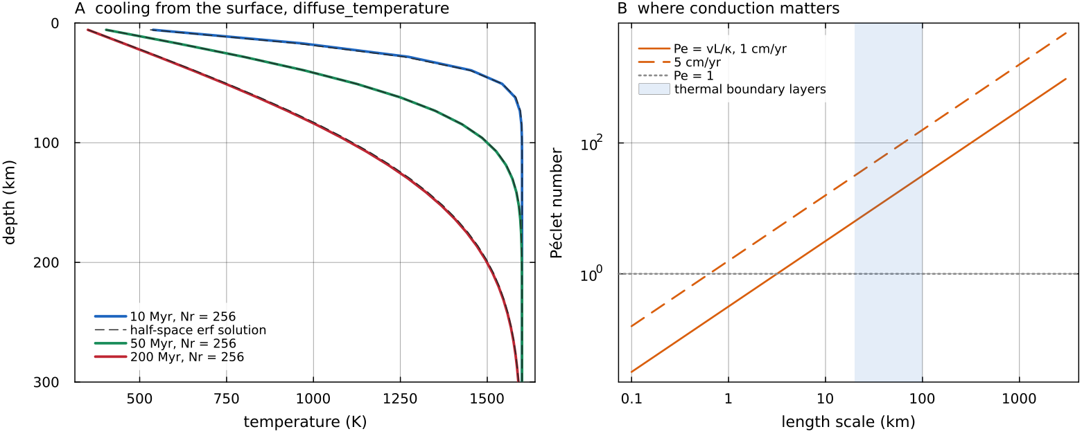
A: diffuse_temperature (Crank-Nicolson, 0.25 Myr steps, 256 radial cells, no flow and no heating) cooling a 1600 K shell from a 300 K surface, against the half-space solution $T_s+(T_m-T_s)\mathrm{erf}(z/2\sqrt{\kappa t})$ at 10, 50 and 200 Myr. B: the Péclet number $vL/\kappa$ against the length scale; across the tens of kilometres of a thermal boundary layer conduction and advection are comparable, while over the depth of the mantle the flow dominates by orders of magnitude. Script: docs/scripts/fig_governing_equations_sections.jl.

Compressibility modes

Rock is compressed by the weight of the rock above it. Along an adiabat, the temperature profile that a parcel follows when it moves without exchanging heat, compression raises the temperature by $dT/dz=\alpha gT/c_p$, and the density of the Earth's mantle rises from about 3400 kg m⁻³ below the crust to about 5600 kg m⁻³ above the CMB (Dziewonski & Anderson 1981). Thermal expansivity falls with compression, by a factor of several across the mantle, while thermal diffusivity tends to rise with depth (Stacey & Davis 2008). The relative size of these effects is measured by the dissipation number $Di$. In the limit $Di\to 0$ the mantle behaves as an incompressible layer and the Boussinesq approximation becomes appropriate, while for $Di$ of order one, as estimated above, adiabatic heating and cooling of moving rock and the frictional heat of viscous flow are comparable with the other terms of the energy equation (Jarvis & McKenzie 1980; Schubert, Turcotte & Olson 2001).

Two consequences follow. A rising parcel cools adiabatically and a sinking one warms, which reduces the temperature contrast that drives the flow; and the work done by buoyancy is dissipated as heat inside the mantle rather than lost. In the anelastic liquid approximation (ALA) these effects are kept by writing every field as a time-independent, radially varying reference state, the adiabat and its density, plus the departure from it that the flow carries. MILEVA builds that reference state from a few parameters, as follows.

cfg.compressibilityMode selects the reference state, through compressibility in physics/compressibility.jl:

mode	reference density	expansivity	diffusivity	adiabatic heating and dissipation
"Boussinesq"	${\rho }_0$	cfg.alpha	cfg.kappa	none
"ALA" (default)	${\rho }_{\text{ref}}(r)$	$\alpha (z)$ linear	$\kappa (z)$	both, if cfg.useShearHeating (default true)
"TALA"	${\rho }_{\text{ref}}(r)$	$\alpha (z)$ linear	$\kappa (z)$	neither

The labels follow common usage with one difference worth knowing. In King et al. (2010) the truncated anelastic liquid approximation (TALA) keeps the adiabatic heating and dissipation of ALA and instead drops the dynamic-pressure contribution to the buoyancy. MILEVA's thermal buoyancy under both ALA and TALA is ${\rho }_{\text{ref}}g\alpha (z)\delta T$, with $\delta T$ the lateral anomaly of $T-T_{\text{ad}}$, to which the compositional and phase terms of compute_buoyancy are added (main_SphCon.jl, step 4). In 2-D both modes also carry the dynamic-pressure term $P{\partial }_r\ln {\rho }_{\text{ref}}$, through the pressure gradient $-{\rho }_{\text{ref}}\mathrm{\nabla }(P/{\rho }_{\text{ref}})$ that the anelastic mass balance requires (below), so in that terminology neither 2-D mode is truncated; the 3-D path has no such term. The MILEVA label "TALA" means the same reference state and mass balance with adiabatic heating and dissipation switched off.

Under ALA and TALA the reference state is the standard anelastic-liquid form, as in King et al. (2010). With depth $z$ and layer thickness $D=R_{\text{out}}-R_{\text{in}}$:

$$\alpha (z)={\alpha }_s+({\alpha }_c-{\alpha }_s)\frac{z}{D},T_{\text{ad}}(z)=T_{\text{pot}}\exp \{\frac{g}{c_p}[{\alpha }_{s}z+({\alpha }_c-{\alpha }_s)\frac{z^2}{2D}]\},$$$${\rho }_{\text{ref}}(z)=max[{\rho }_0(\frac{T_{\text{ad}}}{T_{\text{pot}}}{)}^{1/\mathrm{\Gamma }},{\rho }_0],\kappa (z)={\kappa }_0[1+f_{\kappa }(\frac{z}{D}{)}^2],$$

with ${\alpha }_s$ = cfg.alpha_surf_ref, ${\alpha }_c$ = cfg.alpha_cmb_ref, $T_{\text{pot}}$ = cfg.T_potential_ref and the Grüneisen parameter $\mathrm{\Gamma }$ = cfg.gruneisen (default 1.1), and $f_{\kappa }$ = cfg.kappaDepthFactor (default 0.5; 0 keeps $\kappa$ constant). The density profile is the Adams-Williamson compression along the adiabat for constant $\mathrm{\Gamma }$ (adiabat_temperature, reference_density, thermal_diffusivity), with $z$ measured from cfg.R_out and $D$ = cfg.R_out $-$ cfg.R_in. reference_density is the one profile the buoyancy, the energy sources, the conductivity and the energy budget read. The lithostatic pressure used by the creep and melting laws, including the simple viscosity law compute_viscosity, is mantle_pressure (physics/melt_phase.jl), which integrates this same ${\rho }_{\text{ref}}$, so pressure and density describe one reference state.

The adiabatic heating term is $Q_{\text{ad}}=-{\rho }_{\text{ref}}\alpha gT{V}_r$ with the full temperature $T$, and viscous dissipation is $\mathrm{\Phi }=2\eta \dot{\epsilon }:\dot{\epsilon }=4\eta {\dot{\epsilon }}_{II}^2$. The two are switched on and off together by cfg.useShearHeating, because in a statistically steady layer the volume integral of one balances the other; including only one injects or removes that whole power (main_SphCon.jl, energy source assembly).

Under ALA and TALA the 2-D mass balance is anelastic, $\mathrm{\nabla }\cdot ({\rho }_{\text{ref}}\mathbf{v})=0$, with the pressure gradient as its adjoint and the compressible deviatoric stress (see the 2-D operator section under Momentum and mass). The same mass flux ${\rho }_f{V}_r$ carries temperature on the grid (advect_temperature_2d, advective form ${\rho }_c^{-1}[\mathrm{\nabla }\cdot (\rho \mathbf{v}T)-T\mathrm{\nabla }\cdot (\rho \mathbf{v})]$ over the exact cell measure), the marker hand-back is conservative in the mass-weighted measure $\sum _m{\rho }_{\text{ref}}(r_m)w_m{T}_m$ (delivery_scale), and the net rotation is removed in the frame of zero angular momentum $\int {\rho }_{\text{ref}}r{V}_{\theta }dV$. With these, advection changes $c_p\int {\rho }_{\text{ref}}TdV$ only by round-off on the grid path (tests/test_anelastic_mass_balance.jl). Before, the 2-D continuity was $\mathrm{\nabla }\cdot \mathbf{v}=0$ in every mode, and advection changed that energy at the rate $c_p\int T{V}_r{\partial }_r{\rho }_{\text{ref}}dV$, $-9.3\times {10}^{12}$ W over steps 100 to 200 of the Earth example. The 3-D path still solves $\mathrm{\nabla }\cdot \mathbf{v}=0$ under ALA/TALA, and validate! warns; cfg.useCompressibleStokes, which scaled the 3-D radial fluxes by an invented ramp $1+0.3z/D$ rather than ${\rho }_{\text{ref}}$, is refused. The depth-dependent diffusivity $\kappa (z)$ rises to 1.5 times its surface value at the CMB (docstring of thermal_diffusivity).

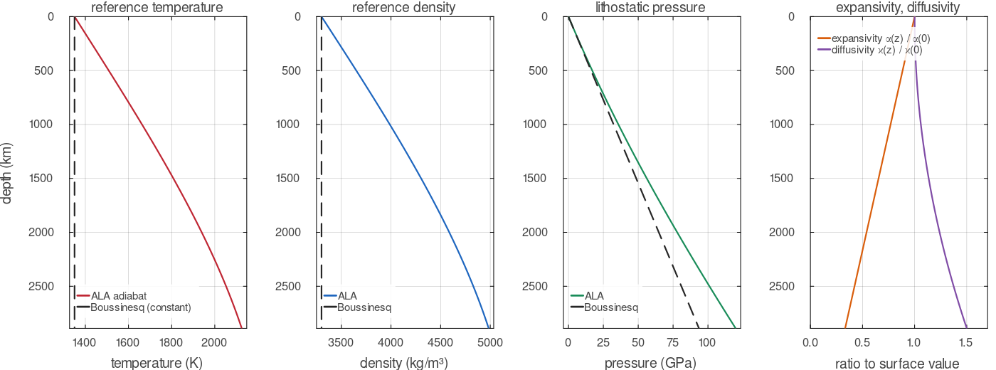
The reference state of the default shell, evaluated by compressibility, mantle_pressure and thermal_diffusivity. Under ALA the adiabat, the Adams-Williamson density and the pressure all rise with depth while the expansivity falls to a third of its surface value; under Boussinesq (dashed) temperature and density are constant and pressure is linear.

Nondimensionalisation and the Rayleigh number

MILEVA takes dimensional input. assemble_stokes converts to nondimensional variables before building the matrix, with the layer thickness $D$, the thermal diffusion time $D^2/\kappa$ and a reference viscosity ${\eta }_{\text{ref}}$ (the median of the viscosity field):

$$\overline{r}=\frac{r}{D},\overline{\mathbf{v}}=\frac{\mathbf{v}D}{\kappa },\overline{P}=\frac{P{D}^2}{{\eta }_{\text{ref}}\kappa },\overline{\eta }=\frac{\eta }{{\eta }_{\text{ref}}},\overline{b}=\frac{b{D}^3}{{\eta }_{\text{ref}}\kappa }.$$

This keeps viscous coefficients of order one and the pressure coefficient of order $1/N_r$, so the condition number is set by the grid rather than by ${\eta }_{\text{ref}}^2$. The solution is converted back with meta.V_scale and meta.P_scale, so the rest of the code never sees the scaled variables.

The thermal Rayleigh number is not an input; it follows from the parameters,

$$Ra=\frac{{\rho }_{0}g\alpha \mathrm{\Delta }T{D}^3}{\kappa \eta },$$

with $\mathrm{\Delta }T$ = temp.T_cmb - temp.T_surf. A benchmark that wants a given $Ra$ sets the viscosity accordingly, as benchmarks/hernlund_tackley_annulus.jl does with $\eta ={\rho }_{0}g\alpha \mathrm{\Delta }T{D}^3/(Ra\kappa )$ on a 1000 km layer. For a temperature-dependent viscosity the reference value must be stated (that driver defines $Ra$ with the viscosity at the mid temperature, as Hernlund & Tackley do). Under ALA the dissipation number $Di=\alpha gD/c_p$ measures the strength of the adiabatic and dissipative terms; it too is derived, not set.

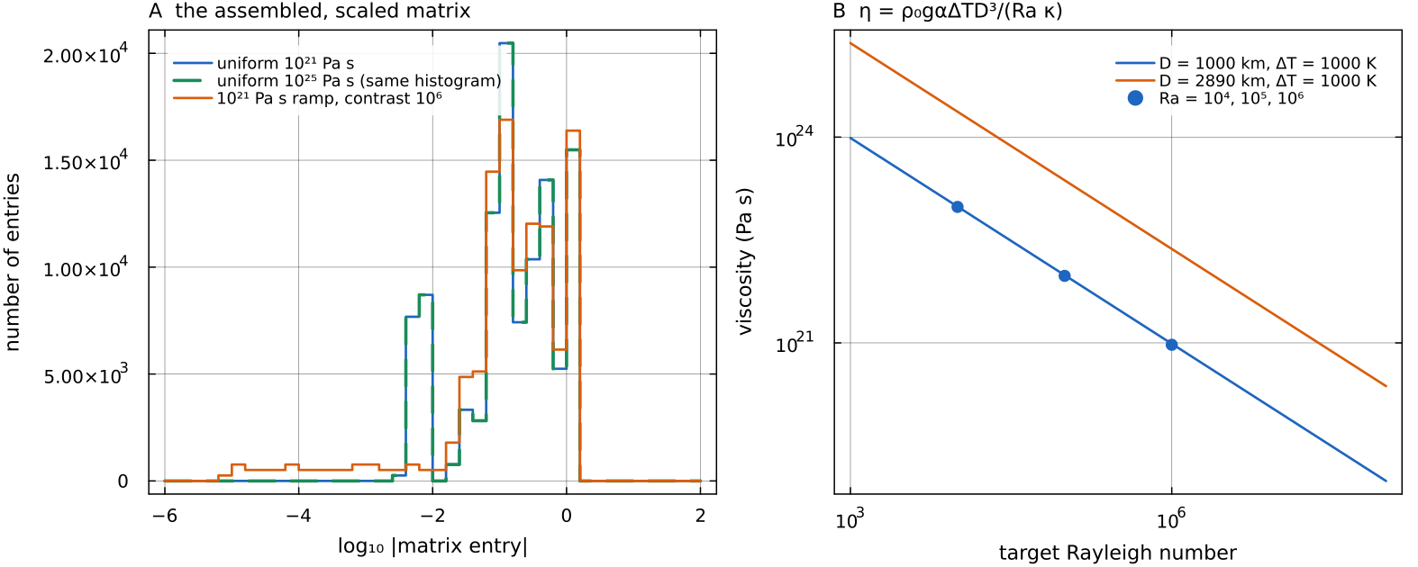
A: the magnitudes of the nonzero entries of the matrix assemble_stokes returns, on a 32 × 128 annulus. A uniform viscosity of ${10}^{21}$ or ${10}^{25}$ Pa s gives the identical matrix, because the scaling divides out ${\eta }_{\text{ref}}$ (only meta.P_scale changes, from 116 Pa to 1.16 MPa); a ${10}^6$ radial contrast spreads the entries by the contrast and no more. B: the viscosity that gives a target $Ra$ on the 1000 km layer of Hernlund & Tackley (2008) and on a 2890 km layer, both with $\mathrm{\Delta }T$ = 1000 K. Script: docs/scripts/fig_governing_equations_sections.jl.

Nonlinear iteration

When the viscosity depends on strain rate, the step solves a fixed point $(\mathbf{v},P,\eta )$. The driver repeats viscosity, Stokes solve and strain rate inside the step until the maximum velocity changes by less than cfg.picardTol (default ${10}^{-4}$), up to cfg.picardMax sweeps. picardMax = 0 (default) means 50 sweeps when a yield law is configured and 1 otherwise. When the change stops decreasing the update is damped in ${\log }_{10}\eta$, which changes the path to the fixed point and not the fixed point. Steps that reach the cap unconverged are counted and logged. The viscosity is rebuilt inside the loop only on the composite path (cfg.useCompositeRheology); the simple Arrhenius path has no strain-rate dependence and converges on the first repeat.

Set picardMax = 1 when viscosity does not depend on strain rate

"Yield law active" means any of mat.maxYieldStress, mat.cohesion_upper, mat.cohesion_lower is finite (main_SphCon.jl), which is true for the default MaterialProperties, so on the simple viscosity path set cfg.picardMax = 1, or set those fields to Inf, to save a repeated Stokes solve per step.

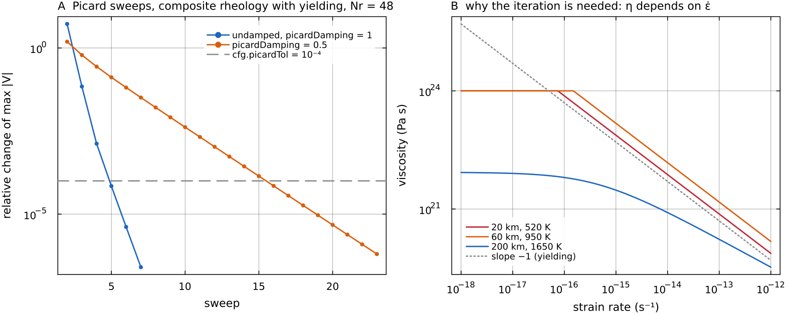
A: the nonlinear iteration of the driver, repeated here on a 48 × 192 annulus with the default composite rheology (yield law active) and a 120 km conductive lid over a plume, each sweep evaluating composite_rheology, solving Stokes, computing the strain rate and applying _picard_viscosity_update. The undamped sweep reaches picardTol in 5 sweeps, a fixed damping of 0.5 in 16. B: why the loop is needed, the composite viscosity against strain rate at three points of the lid and mantle; where the yield branch is active its slope is $-1$. Script: docs/scripts/fig_governing_equations_sections.jl.

Verifying the operator

The work-dissipation identity holds exactly for any Stokes solution at any viscosity field,

$$W=\int \mathbf{b}\cdot \mathbf{v}dV=\int 2\eta \dot{\epsilon }:\dot{\epsilon }dV=D_{\text{visc}},W/D_{\text{visc}}=1,$$

and negative $W$ is impossible because dissipation is positive definite. tests/test_annulus_operator.jl solves a smooth load on an exponential radial viscosity ramp in the spherical annulus at $N_r=32$ and asserts $W>0$ and $|W/D-1|<0.05$ at contrasts $1$ to ${10}^8$, and that the error shrinks with refinement (at contrast ${10}^8$: $W/D=1.0211$ at $N_r=32$ and $|W/D-1|=0.0063$ at $N_r=64$). The same file checks that rigid rotation is annihilated to round-off. For the 3-D operator, tests/test_stokes_3d_variable_eta.jl records on a Yin-Yang chunk with a radial viscosity ramp:

contrast	$N_r=8$	$N_r=12$	$N_r=16$
1	0.9961	1.0026	1.0029
${10}^2$	0.9880	0.9952	0.9985
${10}^4$	0.9909	0.9921	0.9953
${10}^6$	0.9812	0.9813	0.9841

improving with refinement at every contrast. These are internal consistency checks of the discrete operator. Comparison with published convection results is a separate matter, treated with the benchmarks.

The 3-D full-deviatoric operator is selected by cfg.useCurvatureTerms (default true); the false branch is the componentwise scalar Laplacian (tests/test_spherical_operator_nullmode.jl pins both).

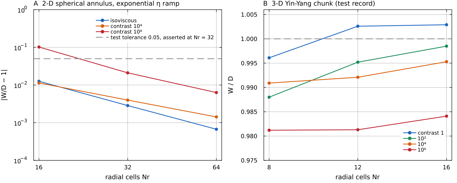
A: $|W/D-1|$ recomputed here for the configuration of tests/test_annulus_operator.jl at 16, 32 and 64 radial cells; at contrast ${10}^8$ it falls from 0.10 to 0.021 to 0.0063, the values quoted above. B: the 3-D values recorded by tests/test_stokes_3d_variable_eta.jl (the table above), plotted, not recomputed. Script: docs/scripts/fig_governing_equations_sections.jl.

Assumptions and simplifications

The equations above are a model of the mantle, not a complete description of it. The approximations MILEVA makes, and the reason for each, are these.

• Infinite Prandtl number. Inertia is dropped from the momentum equation, which is justified by $Re\sim {10}^{-21}$ and makes each Stokes solve independent of the previous velocity.

• Anelastic mass balance in 2-D, incompressible in 3-D. Under ALA/TALA the 2-D annulus solves $\mathrm{\nabla }\cdot ({\rho }_{\text{ref}}\mathbf{v})=0$ with a time-independent ${\rho }_{\text{ref}}$, which filters sound waves; Boussinesq runs keep $\mathrm{\nabla }\cdot \mathbf{v}=0$. The 3-D shell keeps $\mathrm{\nabla }\cdot \mathbf{v}=0$ in every mode (validate! warns under ALA/TALA).

• Buoyancy relative to a reference state. Only departures from the reference density enter $\mathbf{b}$. A density change that is the same everywhere at one radius is balanced by pressure and drives no flow, so the thermal, phase and pile terms are written as lateral anomalies and the other compositional terms affect the flow only through their lateral variation.

• Constant gravity and heat capacity. $g$ = cfg.g and $c_p=1250$ J kg⁻¹ K⁻¹ are the same at every depth. In a real mantle gravity varies by about ten per cent between the surface and the CMB (Dziewonski & Anderson 1981); no self-gravitation of the flow is computed.

• A prescribed reference state. The adiabat, density, expansivity and diffusivity are fixed functions of depth (or a table, see Material tables), not updated from the evolving mean temperature.

• Viscous rock. Elastic stress memory is absent from the momentum equation; viscoelastic behaviour is approximated through an effective viscosity on its own page (Viscoelastoplastic rheology).

• A fixed, flat, free-slip outer surface. Surface topography is treated separately (Free surface and isostasy).

• Two dimensions in the annulus. The spherical annulus reproduces the radial weighting of a sphere, but its flow is two-dimensional, so plumes are sheets and there is no toroidal motion within the shell. The 3-D Yin-Yang shell removes this restriction at much higher cost (Hernlund & Tackley 2008).

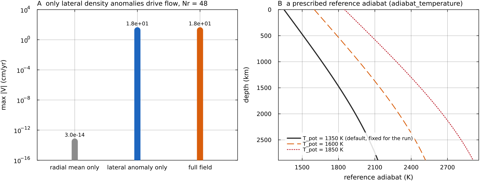
A: the blob buoyancy on a 48 × 192 annulus split into its radial mean and its lateral anomaly, each solved alone. The radial mean drives $3\times {10}^{-14}$ cm/yr, round-off, and the lateral part drives the same 18.1 cm/yr as the full field, so only lateral anomalies matter for the flow. B: the reference adiabat of adiabat_temperature for the default T_potential_ref = 1350 K and two warmer values; the run keeps the one it starts with, whatever its mean temperature does later. Script: docs/scripts/fig_governing_equations_sections.jl.

Where in the code

What	File, function
2-D Stokes assembly, deviatoric operator	solvers/stokes_assembly.jl: assemble_stokes, _viscous_block_deviatoric
3-D Stokes assembly	solvers/stokes_assembly_3d.jl: assemble_stokes_3d
metric exponent and measures	utils/geometry.jl: geometry_exponent, cell_measure, shell_measure
reference state	physics/compressibility.jl: compressibility, adiabat_temperature, thermal_diffusivity, anelastic_density
lithostatic pressure	physics/melt_phase.jl: mantle_pressure
strain rate and invariant	utils/compute_strain_rate.jl: compute_strain_rate
Picard loop, net-rotation removal, source assembly	main_SphCon.jl: main_SphCon, _net_rotation_rate
configuration fields	config/SimConfig.jl: geometry, dim, compressibilityMode, useDeviatoricStress, useCurvatureTerms, removeNetRotation, picardMax, picardTol

Key references

• Jarvis, G. T. & McKenzie, D. P. (1980). Convection in a compressible fluid with infinite Prandtl number. J. Fluid Mech. 96, 515-583. doi:10.1017/S002211208000225X

• Hernlund, J. W. & Tackley, P. J. (2008). Modeling mantle convection in the spherical annulus. PEPI 171, 48-54. doi:10.1016/j.pepi.2008.07.037

• King, S. D. et al. (2010). A community benchmark for 2-D Cartesian compressible convection in the Earth's mantle. GJI 180, 73-87. (Source of the ALA reference-state form; not used as a validation target.) doi:10.1111/j.1365-246X.2009.04413.x

Further reading

• Schubert, G., Turcotte, D. L. & Olson, P. (2001). Mantle Convection in the Earth and Planets. Cambridge University Press. doi:10.1017/CBO9780511612879 The standard monograph on rheology, the governing equations, boundary-layer theory and the thermal history of the terrestrial planets.

• Turcotte, D. L. & Schubert, G. (2014). Geodynamics, 3rd ed. Cambridge University Press. doi:10.1017/CBO9780511843877 Graduate textbook; derivation of the Stokes and energy equations, boundary-layer scaling of convection, mantle viscosity from post-glacial rebound.

• Ricard, Y. (2015). Physics of mantle convection. In Treatise on Geophysics, 2nd ed., vol. 7, 23-71. Elsevier. doi:10.1016/B978-0-444-53802-4.00127-5 A careful treatment of compressibility, the reference state, the anelastic and Boussinesq approximations and the energy budget.

• Jarvis, G. T. & McKenzie, D. P. (1980). Convection in a compressible fluid with infinite Prandtl number. J. Fluid Mech. 96, 515-583. doi:10.1017/S002211208000225X The origin of the anelastic liquid approximation for the mantle.

• Gerya, T. (2019). Introduction to Numerical Geodynamic Modelling, 2nd ed. Cambridge University Press. doi:10.1017/9781316534243 Staggered-grid finite differences, marker-in-cell advection and the coupling of Stokes and energy equations, with worked examples.

• Harlow, F. H. & Welch, J. E. (1965). Numerical calculation of time-dependent viscous incompressible flow of fluid with free surface. Phys. Fluids 8, 2182-2189. doi:10.1063/1.1761178 The staggered (MAC) grid.

• Tackley, P. J. (2008). Modelling compressible mantle convection with large viscosity contrasts in a three-dimensional spherical shell using the yin-yang grid. PEPI 171, 7-18. doi:10.1016/j.pepi.2008.08.005 Compressible convection and large viscosity contrasts on the Yin-Yang shell.

• Stacey, F. D. & Davis, P. M. (2008). Physics of the Earth, 4th ed. Cambridge University Press. doi:10.1017/CBO9780511812910 Thermodynamics of the deep Earth, including adiabats, the Grüneisen parameter, the depth dependence of expansivity and conductivity.

• Dziewonski, A. M. & Anderson, D. L. (1981). Preliminary reference Earth model. PEPI 25, 297-356. doi:10.1016/0031-9201(81)90046-7 Radial density, pressure and gravity of the Earth (PREM).

• Solomatov, V. S. & Moresi, L.-N. (1996). Stagnant lid convection on Venus. J. Geophys. Res. Planets 101, 4737-4753. doi:10.1029/95JE03361

• Nimmo, F. & McKenzie, D. (1998). Volcanism and tectonics on Venus. Annu. Rev. Earth Planet. Sci. 26, 23-51. doi:10.1146/annurev.earth.26.1.23