Examples

The examples/ folder holds runnable drivers that set up a complete model, call the solver and write ParaView output. They are meant to be read as well as run: each file states its physics, its parameters and its run-length knobs in the header, and each sets every optional physics flag explicitly rather than inheriting a default.

Example	Dimension	Driver	Page
Onset of convection: growth rates and the critical Rayleigh number	2-D spherical annulus	examples/annulus_onset_2d.jl	Onset of convection
Isoviscous convection at Ra = 10⁴, 10⁵, 10⁶	2-D spherical annulus	examples/annulus_convection_2d.jl	Isoviscous convection
A plume rising from the core-mantle boundary	2-D spherical annulus	examples/annulus_plume_2d.jl	Plume from the CMB
Boussinesq, TALA and ALA at three dissipation numbers	2-D spherical annulus	examples/annulus_compressible_2d.jl	Boussinesq, TALA and ALA
Purely internal heating with an insulating core at Ra = 10⁴, 10⁵, 10⁶	2-D spherical annulus	examples/annulus_internal_heating_2d.jl	Internal heating
Stagnant lid that fails: Arrhenius viscosity and a yield stress	2-D spherical annulus	examples/annulus_stagnant_lid_2d.jl	Stagnant lid
Whole-mantle or layered convection with an endothermic phase change	2-D spherical annulus	examples/annulus_phase_layering_2d.jl	Phase-change layering
Planform of convection with a stiff lower mantle, four viscosity profiles	2-D spherical annulus	examples/annulus_bunge_2d.jl	Stiff lower mantle
Mobile to stagnant lid: the same shell at viscosity contrasts 1 to 10⁶	2-D spherical annulus	examples/annulus_stagnant_lid_2d.jl	Mobile to stagnant lid
Earth's mantle with a Perple_X reference state and the Steinberger & Calderwood viscosity	2-D spherical annulus	examples/annulus_earth_steinberger_2d.jl	Earth's mantle
Primordial and recycled material in the lower mantle over 4.5 Gyr	2-D spherical annulus	examples/annulus_primordial_recycled_2d.jl	Primordial material
Mobile, episodic, plutonic-squishy and stagnant lids with magmatism over 4.5 Gyr	2-D spherical annulus	examples/annulus_lid_regimes_2d.jl	Tectonic regimes
Mars and Mercury over 4.5 Gyr, with and without a crust (runs in progress)	2-D spherical annulus	examples/annulus_fleury_thermal_evolution_2d.jl	Mars and Mercury
Three continental rafts and three slabs over 1 Gyr	2-D spherical annulus	examples/annulus_continents_2d.jl	Continents
Plume planforms at Ra = 10⁴, 10⁵, 10⁶	3-D Yin-Yang shell, 2 MPI ranks	examples/yinyang_convection_3d.jl	3-D plume planforms

Batch scripts for all of them are in hpc/, described in Running on HPC.

Onset of convection

Isoviscous convection

Plume from the CMB

Boussinesq, TALA and ALA

Internal heating

Stagnant lid

Phase-change layering

Stiff lower mantle

Mobile to stagnant lid

Earth's mantle

Primordial material

Tectonic regimes

Continents

3-D plume planforms

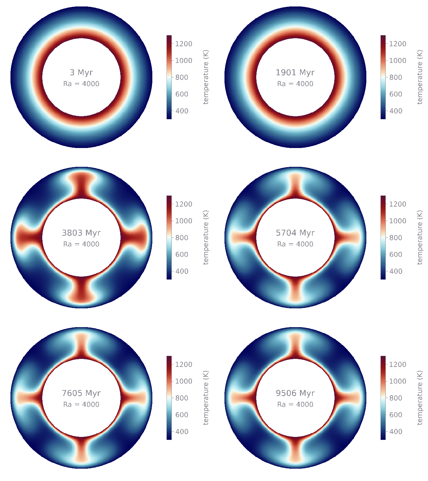
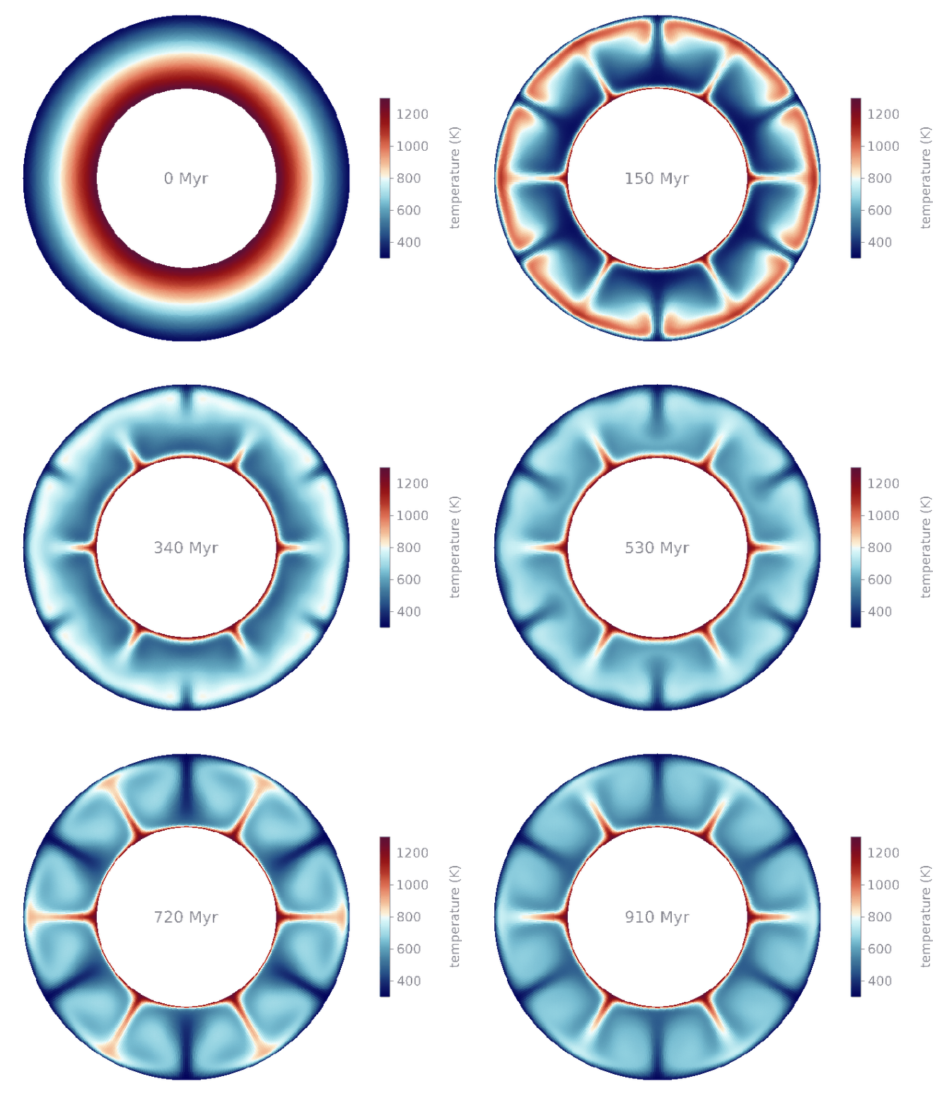
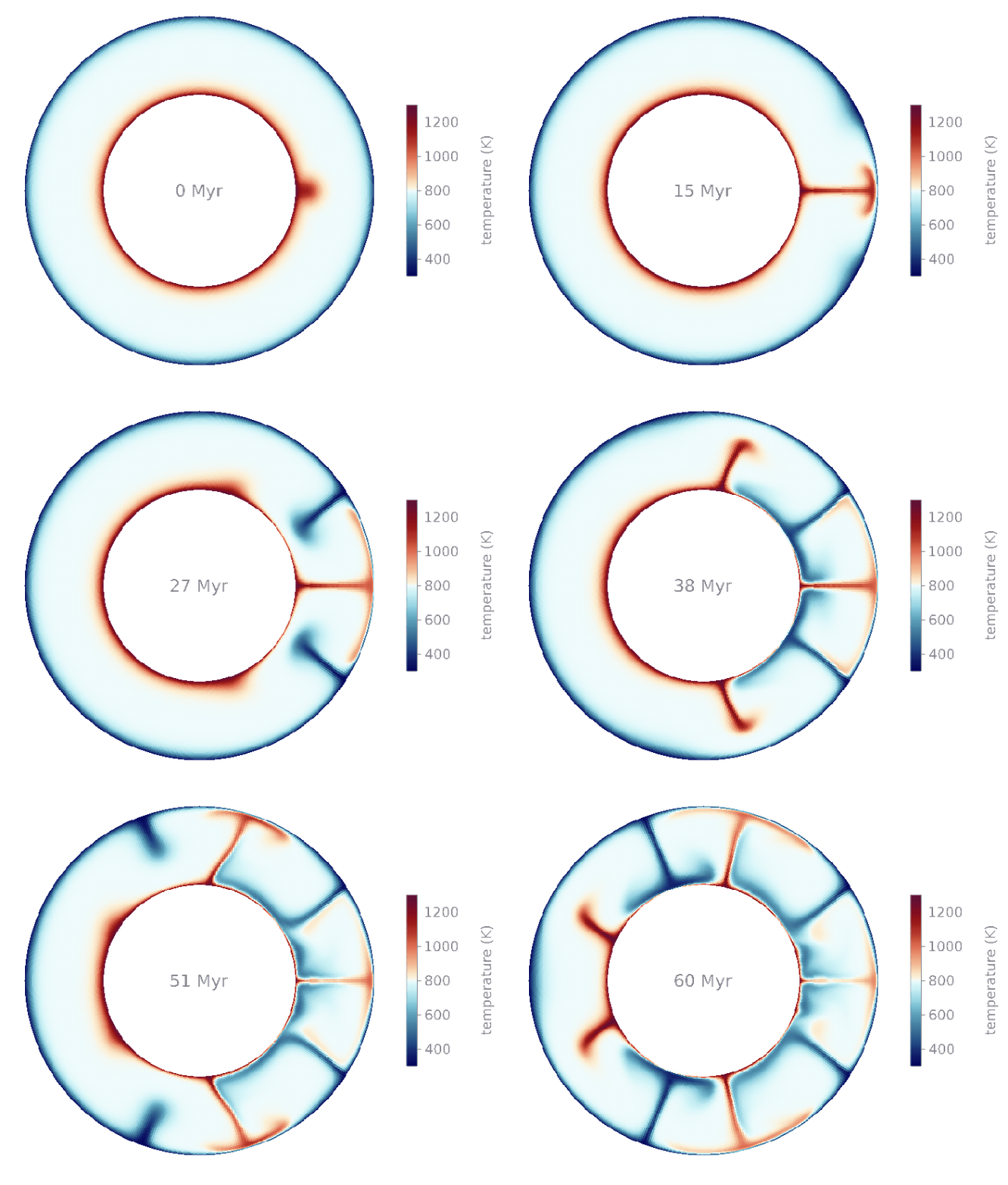
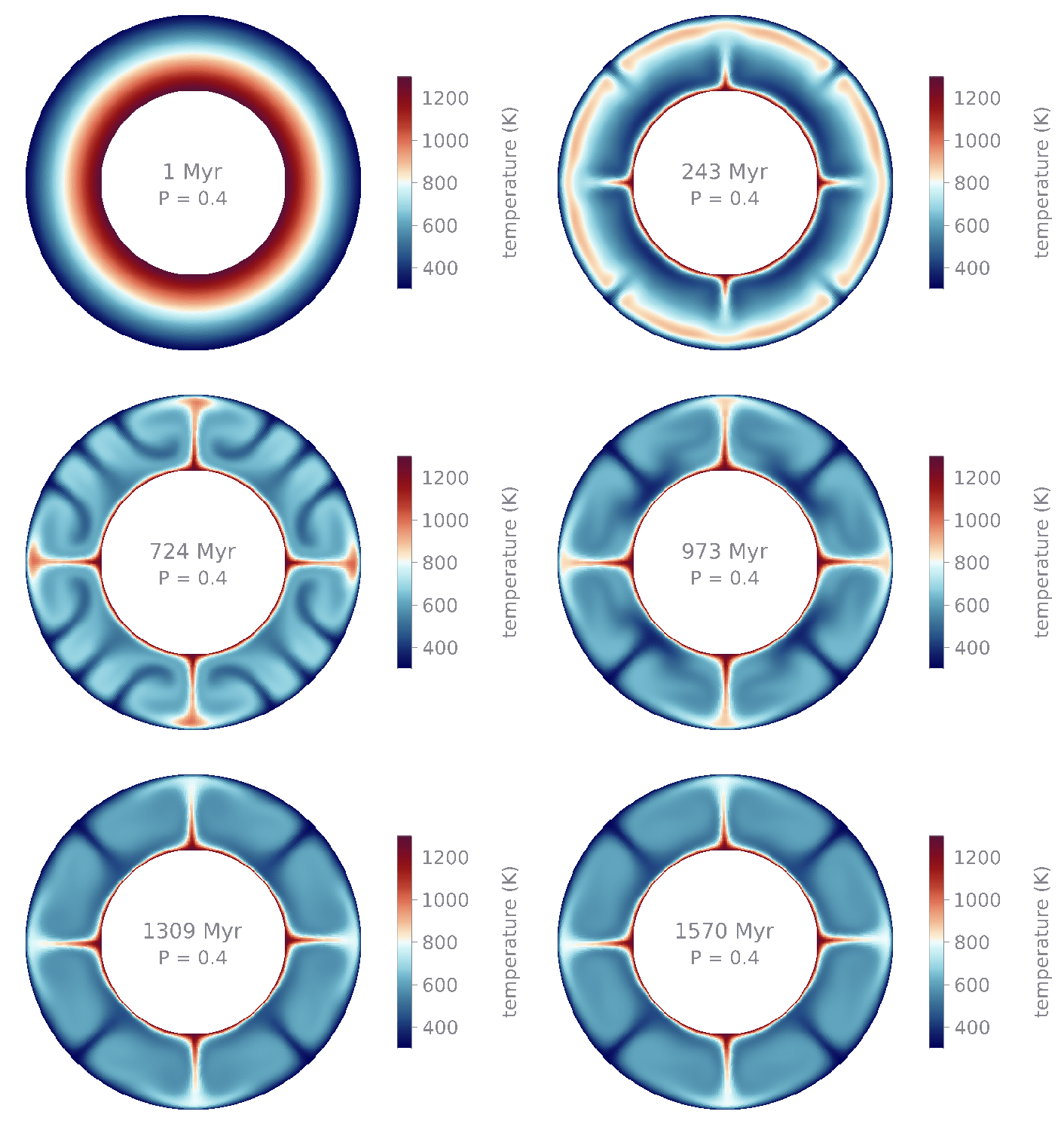
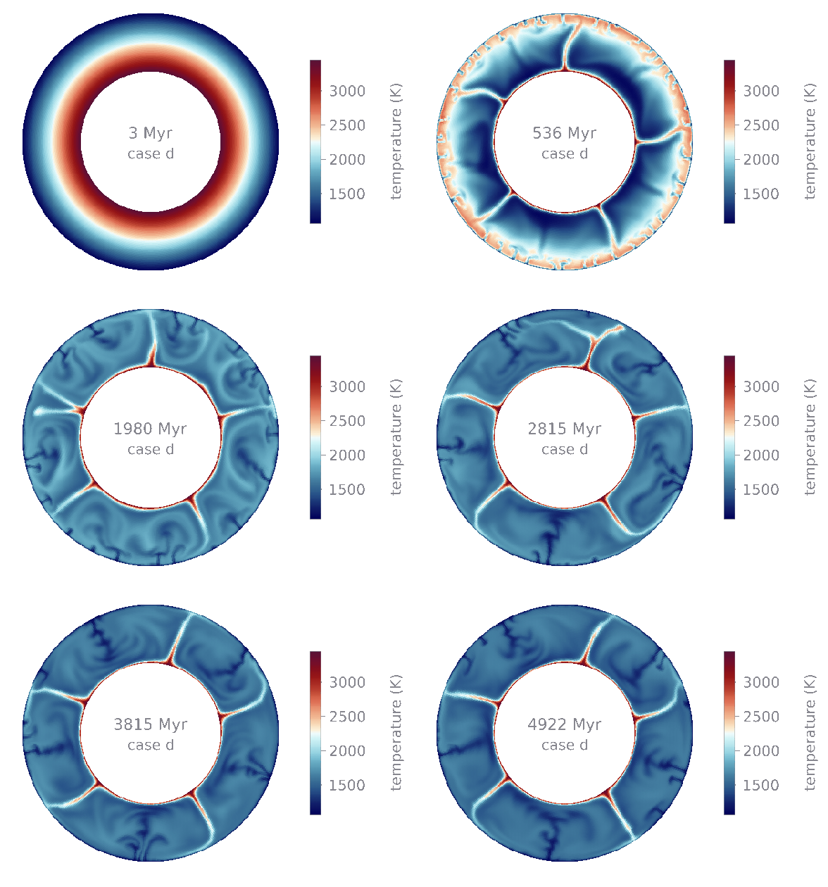
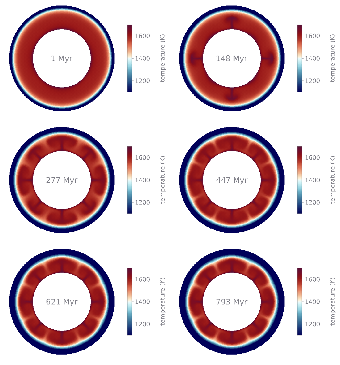
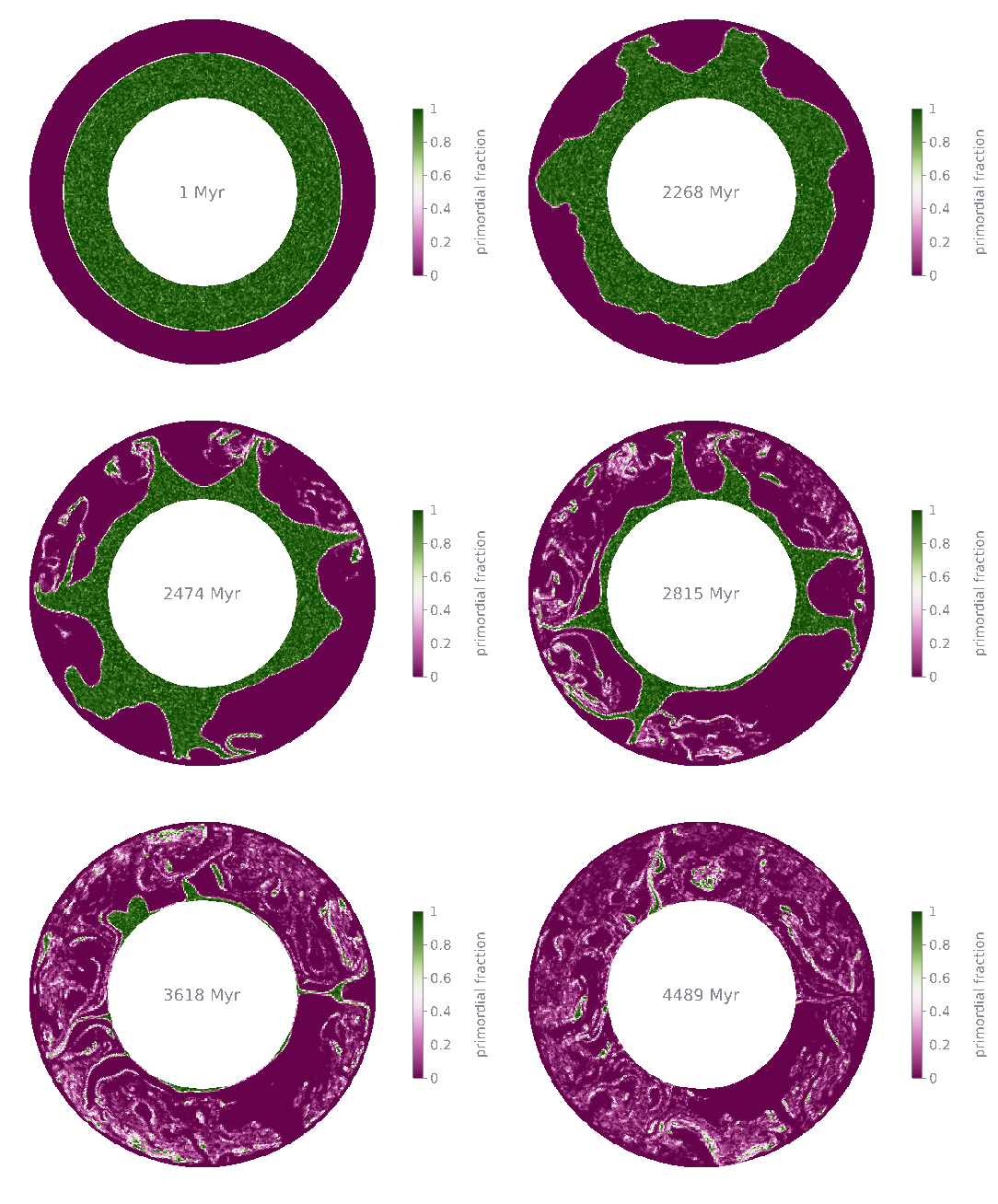
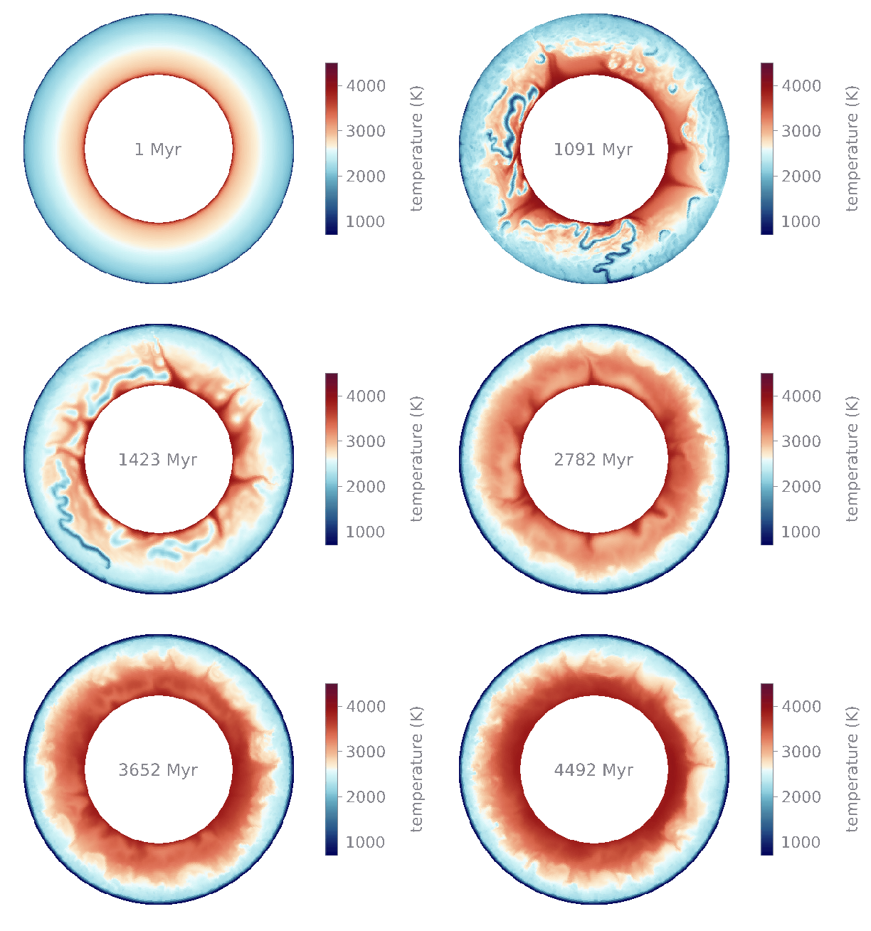
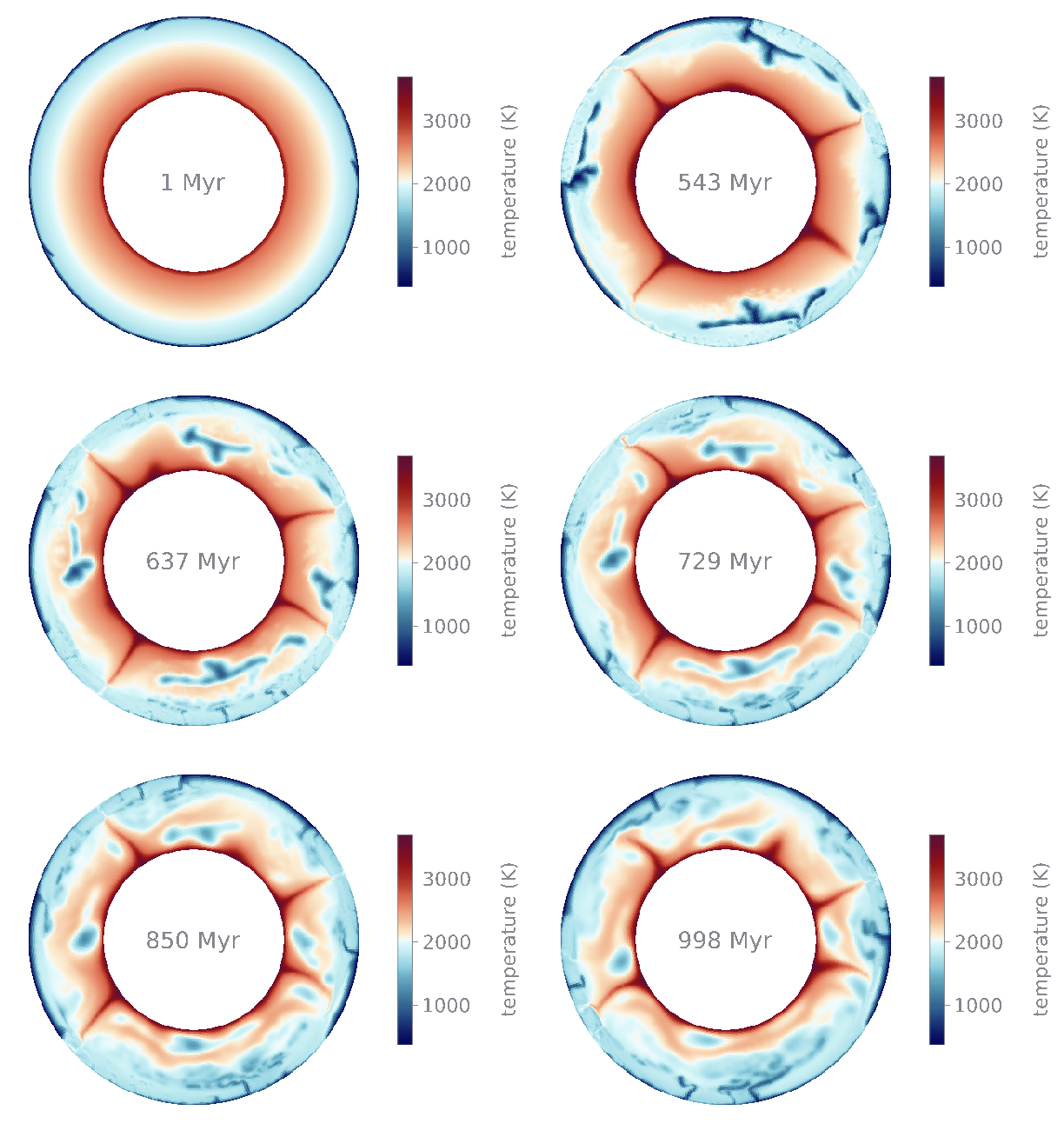
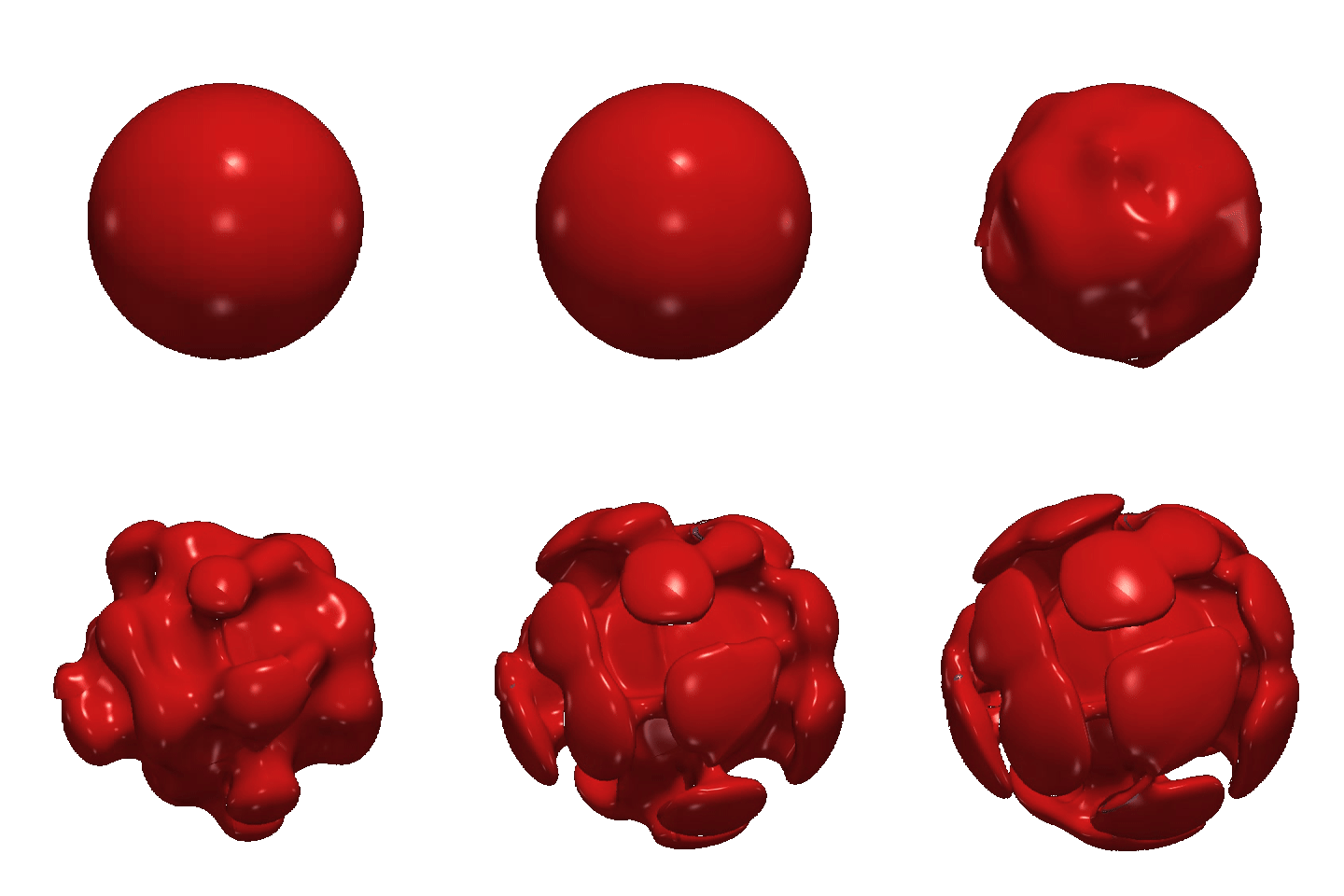
Every example at a glance, in the order of the menu: short preview runs of the 2-D drivers (temperature from cold blue to hot red, except composition for primordial material; grids and run lengths on each page) and the hot-temperature isosurface of the 3-D shell at Ra = 10⁶.

Common conventions

Geometry. Every 2-D example runs in the spherical annulus, cfg.geometry = "spherical_annulus", whose radial measure is $r^{2}dr$, so the core-mantle boundary carries the area ratio of a sphere. All examples use the same shell: $r_i/r_o=1.22/2.22=0.5495$, scaled to a mantle $D=1000$ km thick ($R_{\mathrm{in}}=1220$ km, $R_{\mathrm{out}}=2220$ km). The 3-D example uses the same radii on the Yin-Yang grid. The shared 2-D set-up lives in examples/common_2d.jl:

helper	what it does
ht_shell!(cfg, mat; Nr)	the shell above, uniform radial grid, Nt = 8 Nr
boussinesq_only!(cfg, temp)	clears every optional physics flag, selects Boussinesq, an isothermal CMB, net-rotation removal and MUMPS
eta_for_Ra(Ra, cfg, ΔT)	viscosity for which ${\rho }_{0}g\alpha \mathrm{\Delta }T{D}^3/(\kappa \eta )=\mathrm{Ra}$
set_uniform_eta!(cfg, mat, η)	a constant viscosity on the simple viscosity path
apply_env_overrides!(cfg)	reads MILEVA_MAXSTEPS, MILEVA_MAXTIME_MYR, MILEVA_OUTDIR, MILEVA_VTKEVERY
window_mean, csv_window_mean	time averages over the last third of a run

Rayleigh number. All examples are dimensional runs of a nondimensional problem. With ${\rho }_0=3300$ kg m⁻³, $g=9.81$ m s⁻², $\alpha =3\times {10}^{-5}$ K⁻¹, $\kappa ={10}^{-6}$ m² s⁻¹ and $D=1000$ km, the viscosity

$$\eta =\frac{{\rho }_{0}g\alpha \mathrm{\Delta }T{D}^3}{\kappa \mathrm{Ra}}$$

is $9.7\times {10}^{22}$, $9.7\times {10}^{21}$ and $9.7\times {10}^{20}$ Pa s at $\mathrm{Ra}={10}^4,{10}^5,{10}^6$ for $\mathrm{\Delta }T=1000$ K. The drivers' end-of-run summaries and the 3-D diagnostics_3d.csv give $V_{\mathrm{rms}}$ nondimensionally as $VD/\kappa$; the 2-D diagnostics.csv and log line give cm/yr (Vrms_cmyr, Vsurf_rms_cmyr); $V_{\mathrm{rms}}=100$ in units of $\kappa /D$ is 0.32 cm/yr. Time is given in thermal diffusion times $D^2/\kappa =31700$ Myr.

Resolution. Science runs start at Nr = 64. Coarser grids appear on these pages only as quick smoke tests.

Output. 2-D runs write diagnostics.csv (one row per cfg.logEvery steps, columns defined in utils/diagnostics_csv.jl), VTK frames under vtk/, six-panel figures under figures/ and checkpoints under checkpoints/, all below output/examples/<case>/ unless MILEVA_OUTDIR is set. The 3-D driver writes its own diagnostics_3d.csv, per-patch .vts files with a .vtm per step, and a .pvd collection.

Headless rendering

The 2-D drivers load Plots before include/mileva.jl, as Getting started requires. On a machine without a display, set GKSwstype=nul so the GR backend renders figures off screen.

Cost on a laptop

Measured on the development laptop (Apple M4, 16 GB, 2 Julia threads, 40 steps, VTK and figures included), October 2026:

driver	grid	s/step	peak memory
annulus_convection_2d.jl 1e5 64 6	64 × 512	0.41	2.3 GB
annulus_plume_2d.jl 1e6 64	64 × 512	0.56	2.4 GB
annulus_stagnant_lid_2d.jl 1e6 64 1e4 1e-11 8	64 × 512	0.70	2.7 GB

The number of steps a run needs is set by the CFL condition and the model-time cap, so it differs between examples by orders of magnitude; each page gives the cap. The 3-D example is meant for a cluster; its cost is discussed on its page.