Grids and geometries

MILEVA builds every grid in one place, setup_grid(cfg, temp) in utils/setup_grid.jl, which dispatches on cfg.dim. Two-dimensional runs use a full annulus of $N_r\times N_t$ cells; three-dimensional runs use one or two latitude-longitude patches of $N_r\times N_{\theta }\times N_{\phi }$ cells. Four geometries come out of these two grid builders.

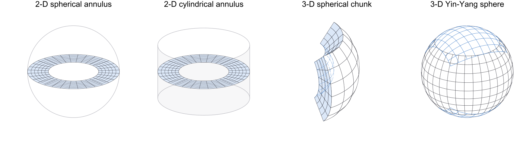
Left to right: the 2-D annulus read as an equatorial slice of a spherical shell and as a cross-section of an infinite cylinder (the mesh is identical, only the metric differs), a 3-D chunk cut from one Yin patch, and the full sphere covered by the Yin (dark) and Yang (blue) patches. Every mesh is the one setup_grid returns. Script: docs/scripts/geometry_figures.jl.

Geometry	cfg.dim	Key settings	Cells	Typical use
2-D spherical annulus	2	geometry = "spherical_annulus" (default)	$N_r\times N_t$	production 2-D runs, parameter studies
2-D cylindrical annulus	2	geometry = "cylindrical_annulus"	$N_r\times N_t$	comparison with cylindrical results
3-D spherical chunk	3	chunkPhiRange < 3π/2, solve with n_schwarz = 0	$N_r\times N_{\theta }\times N_{\phi }$	regional 3-D Stokes problems, operator tests
3-D Yin-Yang sphere	3	default chunkPhiRange = 3π/2	$2\times N_r\times N_{\theta }\times 3N_{\theta }$	whole-mantle 3-D convection

2-D spherical annulus

cfg = SimConfig()
cfg.dim      = 2
cfg.geometry = "spherical_annulus"   # the default
cfg.R_in, cfg.R_out = 3481e3, 6371e3
cfg.Nr, cfg.Nt = 96, 384             # radial and azimuthal cells
cfg.amrStretchFactor = 2.0           # optional: refine both boundary layers

The domain is the full ring $R_{in}\le r\le R_{out}$, $0\le \theta <2\pi$, periodic in $\theta$, with $N_t$ equal cells of width $2\pi /N_t$ and $N_r$ radial cells. The equations carry the spherical-annulus metric of Hernlund & Tackley (2008): every radial integral and divergence uses the measure $r^{2}drd\theta$, so the ring behaves like the equatorial slice of a spherical shell, with the inner-to-outer boundary area ratio of a sphere, $(R_{in}/R_{out}{)}^2$. This is the default and the geometry of every 2-D production run.

The radial axis is uniform when amrStretchFactor is 0 and tanh-stretched otherwise, with the smallest cells at the core-mantle boundary and the surface (see Radial grid stretching). The mesh is the same for both 2-D geometries.

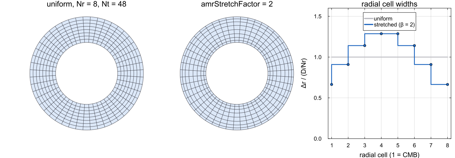
The annulus as setup_grid builds it at $N_r=8$, $N_t=48$ with the default radii: uniform (left) and with amrStretchFactor = 2 (centre). Right: the radial cell widths of both, in units of the uniform width $D/N_r$; stretching makes the two boundary cells about two thirds of the uniform width and the mid-mantle cells about 1.3 times wider.

Boundaries are the two circles: free slip by default, with the temperature fixed at the faces $r=R_{in}$ and $r=R_{out}$. The ring has no lateral walls. Because rigid rotation is a null mode of the annulus Stokes operator, cfg.removeNetRotation = true (the default) removes the net rotation after each solve. Solvers: direct (UMFPACK, MUMPS), BiCGSTAB with AMG, or geometric multigrid, all on the same assembled matrix (see Staggered finite volumes in the annulus).

2-D cylindrical annulus

cfg.geometry = "cylindrical_annulus"   # same mesh, measure r dr dθ

The mesh, the unknowns and the boundary conditions are those of the spherical annulus. One number changes: the exponent $m$ in the shell area $A(r)\propto r^m$, returned by geometry_exponent(cfg) in utils/geometry.jl, is 1 instead of 2. The radial divergence becomes $(1/r){\partial }_r(r\cdot )$, the cell measure $\int rdrd\theta$, and the ring is read as a cross-section of an infinite cylinder.

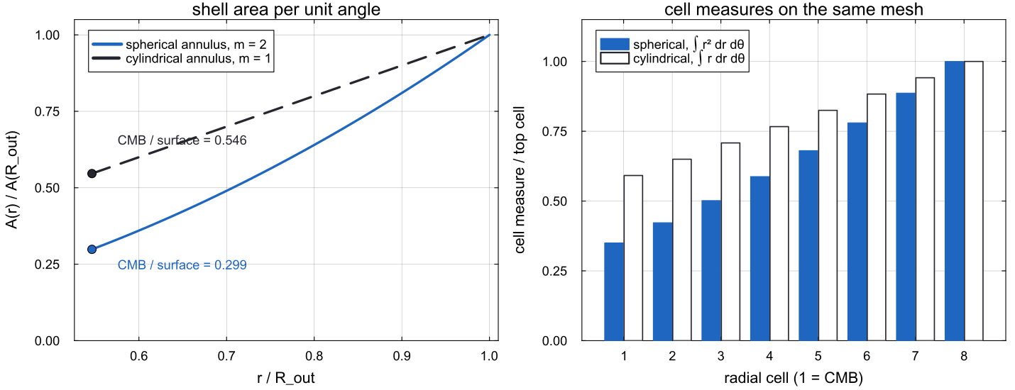
Left: shell area relative to the surface, $(r/R_{out}{)}^m$, for the default radii. The core-mantle boundary has 0.299 of the surface area in the spherical annulus and 0.546 in the cylindrical one. Right: the measure of each radial cell of the $N_r=8$ mesh relative to the top cell, from cell_measure. The deep cells weigh more in the cylinder, so every volume integral (mean temperature, rms velocity, inventories) and every boundary-power balance shifts toward the core.

The area ratio is the consequence that matters most. On a Venus-sized body (3110 / 6052 km) the core boundary has 51 % of the surface area in the cylinder and 26 % in a sphere, so the cylinder delivers basal heat over 1.95 times the relative area. Use the cylindrical annulus to reproduce or compare with cylindrical results; use the spherical annulus for anything that rests on the balance of basal and surface heat flow. The bare spelling "annulus" is refused by validate! because it does not say which.

3-D spherical chunk

cfg = SimConfig()
cfg.dim           = 3
cfg.Nr, cfg.Nt    = 16, 8              # Nt sets the colatitude cells N_θ
cfg.chunkPhiRange = 100π/180           # longitude span, radians
cfg.amrStretchFactor = 2.0             # optional radial refinement
cfg.solverType = "multigrid";  cfg.mgLevels = 2   # 3-D always uses multigrid
grid = setup_grid(cfg, temp)
Vr, Vth, Vph, P, divMax, info = multigrid_stokes(grid, ETA, buoy, cfg; n_schwarz = 0)

A chunk is a single Yin-type patch with a shortened longitude span. cfg.Nt sets $N_{\theta }$ over the fixed colatitude range $45°\le \theta \le 135°$ (latitudes 45° S to 45° N). cfg.chunkPhiRange sets the longitude range, centred on $\phi =0$: the patch spans $-\mathrm{\Phi }/2\le \phi \le \mathrm{\Phi }/2$ with $\mathrm{\Phi }$ = chunkPhiRange, and the longitude cell count is $N_{\phi }=3N_{\theta }\mathrm{\Phi }/(3\pi /2)$, rounded to a multiple of 3, so the angular spacing in $\phi$ stays close to that in $\theta$. A 100° chunk with $N_{\theta }=8$ therefore has $N_{\phi }=9$. The radial axis is the same stretched grid as in 2-D, and $\theta$ and $\phi$ can be stretched as well (amrStretchTheta, amrStretchPhi).

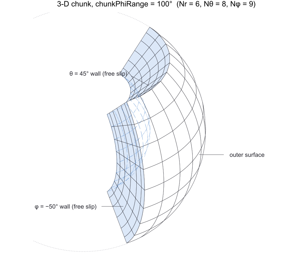
A 100° chunk at $N_r=6$, $N_{\theta }=8$, $N_{\phi }=9$, radially stretched, seen from outside: the outer surface (white), the $\theta =45°$ wall and the $\phi =-50°$ wall (shaded). The core-mantle boundary face, hidden behind them, is drawn dashed.

Boundary conditions, from assemble_stokes_3d with no Schwarz data supplied: the four side walls are impermeable ($V_{\theta }=0$ on the $\theta$ walls, $V_{\phi }=0$ on the $\phi$ walls) and free slip (the shear traction on them is zero); the outer surface and the core-mantle boundary are free slip as in the full shell. Because a chunk has no partner patch, the Yin-Yang Schwarz iteration must be off: call the 3-D multigrid_stokes with n_schwarz = 0.

The chunk is a geometry of the 3-D grid and Stokes solver. It is what tests/test_stokes_3d_operator_consistency.jl and tests/test_vcycle_var_eta.jl (100° chunks) and tests/test_stretched_radial_3d.jl (90° chunks) solve on. The time loop in main_SphCon.jl always runs the coupled Yin-Yang solve, and the 3-D temperature solver treats $\phi$ as periodic, so a time-dependent chunk calculation is not a run mode of the main loop. With MPI, chunkPhiRange enters only the count $N_{\phi }$ used to size the decomposition (_nph_3d in parallel/mpi_init.jl); the MPI layout is always a Yin and a Yang patch.

3-D Yin-Yang sphere

cfg = SimConfig()
cfg.dim        = 3
cfg.Nr, cfg.Nt = 32, 24               # N_θ per patch; N_φ = 3 N_θ = 72
cfg.amrStretchFactor = 2.0
cfg.solverType = "multigrid";  cfg.mgLevels = 2
cfg.δ_yy = 0;  cfg.useMinOverlapGrid = false   # basic-overlap grid

With the default chunkPhiRange = 3π/2 each patch spans $45°\le \theta \le 135°$ and $-135°\le \phi \le 135°$ with $N_{\phi }=3N_{\theta }$. Two such patches, Yin and Yang, are joined by the Kageyama & Sato (2004) rotation $(x,y,z)\to (-x,z,y)$ and together cover the sphere without poles. They are coupled by a Schwarz iteration that exchanges velocity and pressure across the seam each Stokes solve. The free-slip surface and core-mantle boundary are the only physical boundaries.

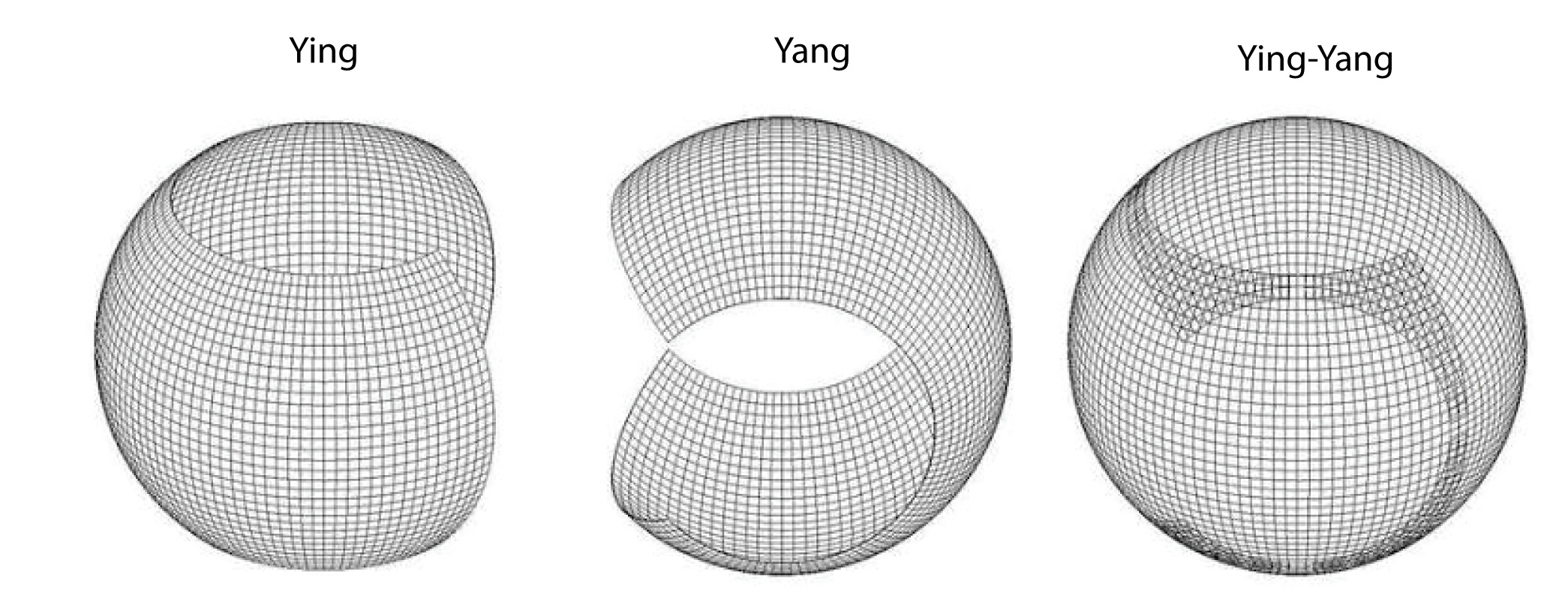
The Yin patch, the Yang patch and the two together. Construction, the transform, the Schwarz coupling and the overlap are described in Yin-Yang grid (3-D).

This is the geometry of the 3-D time loop and of the MPI drivers, which run 2 x mpiNr x mpiNt x mpiNp ranks, half on each patch (see Parallel solvers (MPI)).

Choosing a geometry

• For 2-D work use the spherical annulus. It is the default, and its boundary area ratio is that of a sphere.

• Switch to the cylindrical annulus only to compare with cylindrical results; report which metric a number was computed with.

• For whole-mantle 3-D convection use the Yin-Yang sphere.

• Use a chunk for regional 3-D Stokes problems solved directly with multigrid_stokes(...; n_schwarz = 0), not for time-dependent runs.

• In 3-D always use solverType = "multigrid" with mgLevels of at least 2; a direct factorisation of the 3-D system does not fit in workstation memory beyond small grids.

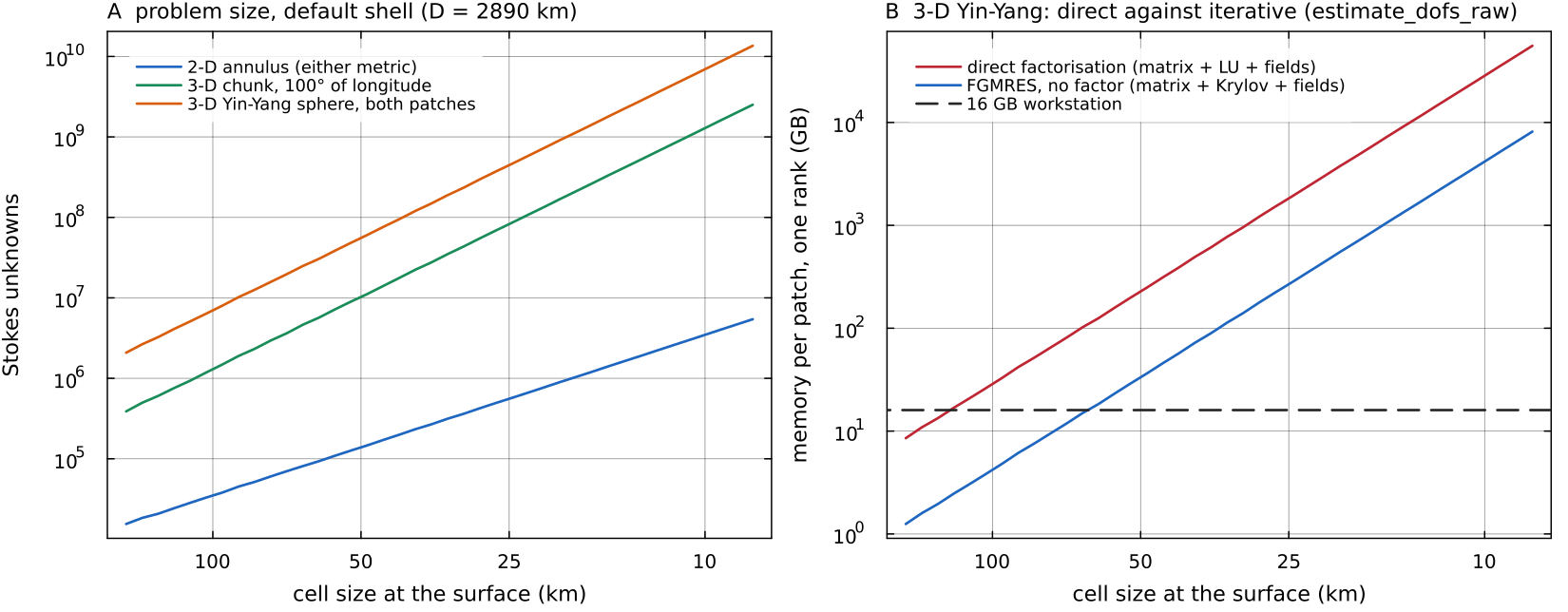
What the choice costs. Left: the number of Stokes unknowns for the default shell when the cell size at the surface is the same in every direction, from the staggered layouts of the two grid builders; at 50 km the 2-D annulus has about $1.5\times {10}^5$ unknowns, a 100° chunk $1.1\times {10}^7$ and the Yin-Yang sphere $6\times {10}^7$. Right: memory per Yin-Yang patch on one rank as estimated by estimate_dofs_raw; a direct factorisation passes 16 GB already near 100 km cells, the iterative path near 60 km, beyond which the 3-D sphere needs several ranks per patch. Script: docs/scripts/fig_numerics_geometries_sections.jl.

Where in the code

What	File	Function
grid factory	utils/setup_grid.jl	setup_grid, _setup_grid_2d, _setup_grid_3d
radial and angular stretching	utils/setup_grid.jl	_amr_radial_grid, _amr_angular_grid
2-D metric exponent and measures	utils/geometry.jl	geometry_exponent, shell_measure, cell_measure, geometry_area_ratio
geometry validation	config/SimConfig.jl	validate!
chunk span and $N_{\phi }$	config/SimConfig.jl, utils/setup_grid.jl, parallel/mpi_init.jl	chunkPhiRange, _setup_grid_3d, _nph_3d
Yin-Yang transforms	utils/setup_grid.jl, utils/yy_interp.jl	yy_yin_to_yang, yy_yang_to_yin
3-D Stokes, chunk or coupled	solvers/multigrid_stokes.jl	multigrid_stokes (n_schwarz)