Geometric multigrid

solvers/multigrid_stokes.jl holds MILEVA's geometric multigrid for the coupled Stokes system $[\mathbf{V};P]$, in two forms:

• 2-D annulus, multigrid_stokes(::MutableGrid2D, ...): flexible GMRES right-preconditioned by one V-cycle. Selected with cfg.solverType = "multigrid". It is an alternative to the direct solvers, which are faster at typical 2-D sizes.

• 3-D Yin-Yang patch, multigrid_stokes(::MutableGrid3D, ...): flexible GMRES right-preconditioned by one V-cycle, inside the Yin-Yang Schwarz iteration. This is the 3-D Stokes path.

Viscosity contrast. In 3-D this is the solver that carries MILEVA to a viscosity contrast of ${10}^{18}$: FGMRES around the V-cycle converges at every contrast from 1 to ${10}^{18}$ in 28 to 73 iterations, with fewer iterations at high contrast, because face viscosities are averaged geometrically and the pressure prolongation is matrix dependent (both below). The 2-D multigrid reaches ${10}^{12}$ on a mid-depth step; see the overview for both.

Both act on the whole saddle-point system with a coupled box smoother rather than on the velocity block alone. The method combines the ingredients described for spherical mantle convection by Tackley (2008): a symmetric coupled smoother, Galerkin coarse operators, geometric viscosity averaging and matrix-dependent pressure interpolation. The multigrid components themselves are standard (Trottenberg et al. 2001).

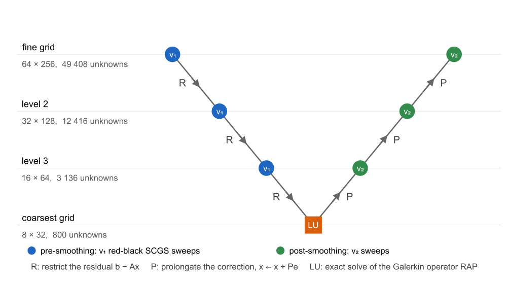
One V-cycle. Down the left leg each level is smoothed and its residual restricted; the coarsest level is solved exactly; up the right leg the correction is prolongated and smoothed again. The level sizes are those MILEVA builds for a 64 × 256 annulus with cfg.mgLevels = 4 (_coarsen_grid); the 3-D hierarchy is built the same way per patch. Script: docs/scripts/solvers_vcycle_schematic.jl.

The SCGS smoother

The smoother is symmetric coupled Gauss-Seidel (SCGS). For each pressure cell it collects the unknowns of that cell, the pressure and the velocities on its faces, and solves the small local saddle-point block exactly:

	Local block	Size
2-D (_scgs_smooth_2d)	$V_{r,i},V_{r,i+1},V_{\theta ,j},V_{\theta ,j+1},P$	5 × 5
3-D (_scgs_smooth_3d)	two faces each of $V_r$, $V_{\theta }$, $V_{\phi }$, and $P$	7 × 7

Cells are swept in red-black order ($(i+j)$ or $(i+j+k)$ parity), so cells of one colour share no unknowns and are updated in parallel with threads. Corrections are relaxed with $\omega =0.7$ (the 2-D omega keyword; in 3-D the module setting _scgs_omega_setting[]). The cell carrying the pressure pin is skipped, since its pressure row is an identity row.

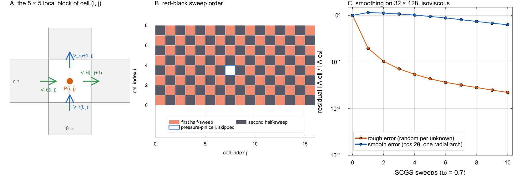
(A) The unknowns updated together for one pressure cell of the 2-D staggered grid. (B) Red-black order on an 8 × 16 corner of the grid; the cell carrying the pressure pin (here at $(N_r/2,N_t/2)$ of an 8 × 16 grid) is skipped. (C) _scgs_smooth_2d applied to $Ae=0$ on the isoviscous 32 × 128 annulus: a rough initial error loses 98 % of its residual in ten sweeps, a smooth one less than half. Removing the smooth part is the job of the coarse levels. Script: docs/scripts/solvers_multigrid_sections.jl.

The 3-D smoother allocates nothing per cell: each thread keeps preallocated 7-entry buffers, fills the local block by walking the sparse columns directly, and solves it with an inline partial-pivoting elimination (_gauss_solve_small!). Together with right-hand-side-only reassembly in the Schwarz loop (assemble_stokes_3d(...; rhs_only = true)) a two-rank run at $N_r$ = 24, $N_{\theta }$ = 40, $N_{\phi }$ = 120 takes 11.5 s per step.

The smoother relies on the exact $G=-B^{\mathsf{T}}$ structure of the finite-volume assembly (see Discretisation).

Hierarchy and coarse operators

Each coarser level halves every grid dimension. In 2-D coarsening continues while $N_r$ and $N_t$ are even and the coarse grid is at least $4\times 8$, up to cfg.mgLevels levels; in 3-D it continues while each halved dimension is at least 2.

Coarse operators are Galerkin products,

$$A_{\ell +1}=R_{\ell }{A}_{\ell }{P}_{\ell },$$

never re-discretised, so the coarse levels keep the spectrum of the fine operator on the curved grid. The transfer operators are built per staggered component (_build_prolongation_2d, _build_prolongation_matrix_3d, _build_restriction_matrix_3d): each velocity component is injected on coarse faces aligned with fine faces and interpolated linearly along its own direction to the faces in between, and is constant across the face. The flux through each coarse face is then the sum of the fine fluxes, so the coarse continuity rows are a true coarse divergence. Pressure is constant over the fine cells of a coarse cell. In 2-D the restriction is the transpose of the prolongation, the radial weights follow the actual face radii (a stretched grid coarsens to a stretched grid), and wall velocities and the two pins take no coarse correction. The coarsest level is solved exactly by sparse LU, factorised once per solve. In 3-D that factor is cached and rebuilt only when the grid changes or the coarse viscosity moves by more than 1 %.

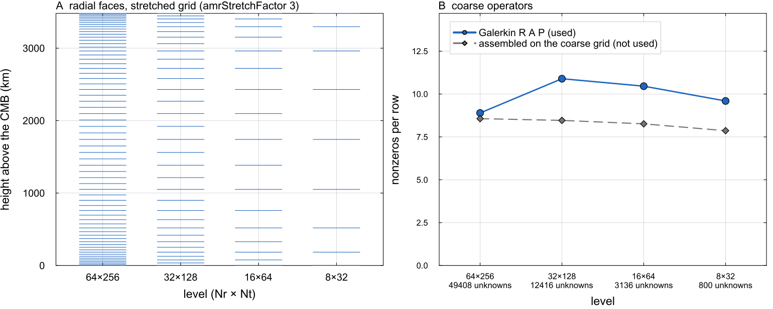
(A) Radial faces of the four levels MILEVA builds (_coarsen_grid) for a 64 × 256 annulus stretched with amrStretchFactor = 3: every coarse face is a fine face, so the refinement at both walls survives to the coarsest level. (B) Nonzeros per row of the Galerkin operators $RAP$ (_galerkin_coarse_2d) for a ${10}^6$ viscosity step, against an operator assembled directly on each coarse grid with the averaged viscosity. The Galerkin product is somewhat denser, which is the price of keeping the fine operator's spectrum. Script: docs/scripts/solvers_multigrid_sections.jl.

Large viscosity contrast

Two choices keep the cycle effective when the viscosity varies by many orders of magnitude.

Geometric viscosity averaging. The 3-D momentum stencil needs viscosities at velocity faces and cell edges, where none is stored. With cfg.useGeometricEta = true (default) they are geometric means of the neighbouring cell values, $\sqrt{{\eta }_a{\eta }_b}$ for two cells and $({\eta }_a{\eta }_b{\eta }_c{\eta }_d{)}^{1/4}$ for four, instead of arithmetic means. An arithmetic mean across a sharp step is dominated by the stiff side, which makes the discrete operator much stiffer near the step than either material; the geometric mean is the natural average for a quantity that varies exponentially. At constant viscosity the two are identical.

Matrix-dependent pressure interpolation (3-D). The pressure prolongation weights each fine cell in a $2\times 2\times 2$ block by its viscosity,

$$P_{\text{fine}}=\frac{8{\eta }_{\text{fine}}}{\sum _{\text{block}}{\eta }_{\text{fine}}}{P}_{\text{coarse}},$$

which reduces to injection at constant viscosity. It is on by default and can be disabled for comparison with MILEVA_NO_MDPI=1. Because the cycle is used inside FGMRES, its effect on iteration counts is small; it matters most when multigrid runs without a Krylov wrapper.

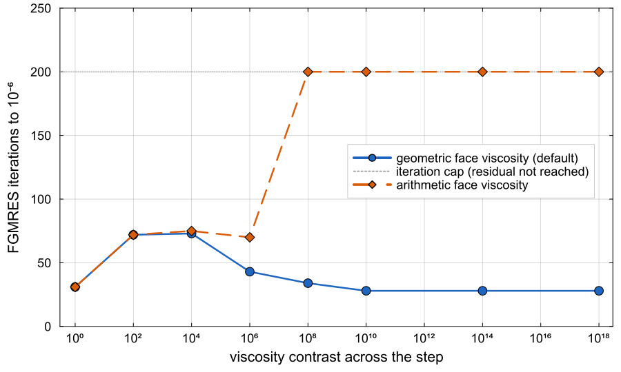
FGMRES iterations (last Schwarz round) to a relative residual of ${10}^{-6}$ for one Yin-Yang shell at $N_r=N_{\theta }=12$, $N_{\phi }=36$, two levels, with a mid-depth viscosity step of the given contrast. Script: docs/scripts/solvers_3d.jl, the setup of tests/test_mdpi_eta_contrast.jl.

Up to a contrast of ${10}^4$ the two averages behave alike. Beyond it the geometric mean needs fewer iterations as the contrast grows (43 at ${10}^6$, 28 from ${10}^{10}$ to ${10}^{18}$), while the arithmetic mean needs 70 at ${10}^6$ and from ${10}^8$ on does not reach the tolerance within the 200-iteration cap (final residuals $4\times {10}^{-3}$ to $0.3$).

Two details that decide convergence

Point pressure pin. The pressure null space is fixed by a single identity row, not by a dense "mean pressure = 0" row. A local smoother cannot relax a row that couples every pressure unknown, and Galerkin coarsening represents it badly. All multigrid calls assemble with point_pin = true.

BC lift. Identity rows (Dirichlet walls, pins and, in 3-D, Schwarz wall values) are detected once per assembly (_bc_lift_initial_guess_2d!; in 3-D the rows whose only nonzero is the diagonal), and the initial guess is set to $x_0[i]=b[i]$ there. The SCGS smoother skips those rows and a Galerkin coarse level only sees a local average of fine boundary values, so without the lift the initial boundary residual would persist.

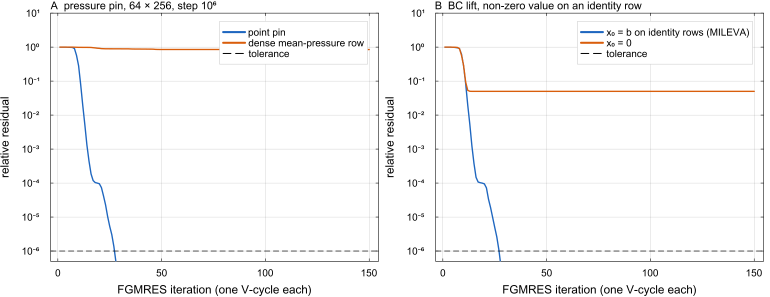
The 2-D FGMRES + V-cycle of multigrid_stokes rebuilt from its parts, so that one ingredient changes at a time; 64 × 256 annulus, four levels, mid-depth viscosity step of ${10}^6$. (A) With the dense mean-pressure row the iteration stalls at a residual near 1; with the point pin it converges in 28 iterations. (B) The pin row given a non-zero value (5 % of $\Vert b\Vert$), standing in for the non-zero wall values of a Schwarz round. Started from $x_0=0$ the residual stops at that value, because no V-cycle ever changes an identity-row unknown; with the lift it converges as before. Script: docs/scripts/solvers_multigrid_sections.jl.

2-D: FGMRES around the V-cycle

In 2-D, FGMRES (restart 50) iterates until the relative residual falls below cfg.krylovTol, at most cfg.krylovMaxIter iterations, each preconditioned by one V-cycle with cfg.mgSmooth pre- and post-sweeps. The Galerkin operators are formed from the unscaled operator and row-equilibrated level by level for the smoother. The same cycle used on its own as a stationary iteration is not a contraction at every depth and contrast; inside FGMRES it converges at 2 to 5 levels.

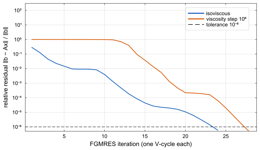
Residual history of the 2-D multigrid on the spherical annulus $f=0.5$, $N_r\times N_t=32\times 128$, four levels, two SCGS sweeps, for the sinker load of tests/test_2d_vcycle_scgs.jl. Each iteration is one V-cycle; the ${10}^6$ step costs four more iterations than the isoviscous shell. Script: docs/scripts/solvers_2d.jl.

Problem	Iterations to ${10}^{-6}$	$max|V_{\text{MG}}-V_{\text{MUMPS}}|/V_{\text{max}}$
isoviscous	24	$6.5\times {10}^{-6}$
viscosity step ${10}^6$	28	$7.4\times {10}^{-9}$

A residual of ${10}^{-6}$ is not a direct solve: on the isoviscous case the largest non-dimensional divergence was $3.6\times {10}^{-1}$ for multigrid against $5\times {10}^{-8}$ for MUMPS, so tighten cfg.krylovTol if divergence matters. At typical 2-D sizes the direct solvers are about ten times faster (see the overview). At 64 × 256 the solver converges with 2, 3 and 4 levels on the isoviscous shell and on a ${10}^6$ step (14 to 29 iterations, tests/test_2d_vcycle_scgs.jl), and up to a contrast of ${10}^{12}$ on a mid-depth step; a thin stiff lid is the case it handles poorly (see the overview).

3-D: FGMRES around the V-cycle

Inside each Schwarz round, each patch is solved by right-preconditioned flexible GMRES (Saad 1993; _gmres_right_precond_3d) with one V-cycle (_vcycle_3d!) as the preconditioner. FGMRES stores the preconditioned vectors $z_j=M^{-1}{v}_j$, which a preconditioner that is itself an iteration requires. Settings:

Setting	Value	Source
Tolerance	cfg.krylovTol (default ${10}^{-8}$)	relative residual
Iteration cap	cfg.krylovMaxIter (default 200)	total inner iterations
Restart	$min(\mathtt{\text{krylovMaxIter}},50)$
Pre/post SCGS sweeps	5 / 5 (serial multigrid_stokes; the one-rank-per-patch MPI path multigrid_stokes_mpi! uses 2 / 2)	fixed in the driver, not cfg.mgSmooth
Levels	cfg.mgLevels (default 4), at least 2 required

The driver logs, at the log cadence, the FGMRES iteration count and residual of the last Schwarz round and every Schwarz residual ([stokes 3-D] lines), so a run whose FGMRES hits its cap is visible in the log. A direct-LU against V-cycle comparison at $N_r$ = 24, $N_{\theta }$ = 16, $N_{\phi }$ = 48 agreed to $max|\mathrm{\Delta }V|/V_{\text{max}}=4.7\times {10}^{-5}$ on both patches.

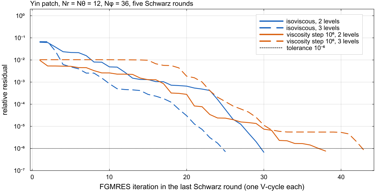
Residual history of the Yin patch in the fifth Schwarz round of multigrid_stokes(::MutableGrid3D, ...), $N_r=N_{\theta }=12$, $N_{\phi }=36$, FGMRES tolerance ${10}^{-6}$, with two and three levels, isoviscous and with a mid-depth viscosity step of ${10}^6$. The round starts from the previous round's solution, so its first residual is already below one. All four cases converge in 25 to 43 iterations; on a grid this small a third level saves little. Script: docs/scripts/solvers_multigrid_sections.jl.

Iteration cap

At $N_r\ge 32$ with strongly temperature-dependent viscosity, FGMRES can need more than 300 iterations to reach ${10}^{-6}$, although the velocity has by then settled to its first two significant figures. Raise cfg.krylovMaxIter (for example to 500) if the log shows capped solves.

Where in the code

Topic	File	Function
2-D driver and V-cycle	solvers/multigrid_stokes.jl	multigrid_stokes(::MutableGrid2D, ...), _vcycle!
3-D driver and V-cycle	solvers/multigrid_stokes.jl	multigrid_stokes(::MutableGrid3D, ...), _vcycle_3d!
Smoothers	solvers/multigrid_stokes.jl	_scgs_smooth_2d, _scgs_smooth_3d, _gauss_solve_small!
Transfers, MDPI	solvers/multigrid_stokes.jl	_build_prolongation_2d, _galerkin_coarse_2d, _build_prolongation_matrix_3d, _build_restriction_matrix_3d
Geometric averaging	solvers/stokes_assembly_3d.jl	_avg2, _avg4 (cfg.useGeometricEta)
FGMRES	solvers/multigrid_stokes.jl	_gmres_right_precond_3d
Tests	tests/	test_2d_vcycle_scgs.jl, test_vcycle_var_eta.jl, test_mdpi_eta_contrast.jl, test_vcycle_visc_contrast_sweep.jl, smoke_stokes_3d_mg.jl

References

• Saad, Y. (1993), A flexible inner-outer preconditioned GMRES algorithm, SIAM J. Sci. Comput. 14, 461-469.

• Tackley, P. J. (2008), Modelling compressible mantle convection with large viscosity contrasts in a three-dimensional spherical shell using the yin-yang grid, Phys. Earth Planet. Inter. 171, 7-18.

• Trottenberg, U., Oosterlee, C. W. and Schüller, A. (2001), Multigrid, Academic Press.