Plume from the CMB (2-D)

A single hot anomaly placed just above the core-mantle boundary rises through the spherical annulus as a plume: a head that grows by entraining the surroundings, a conduit that trails it back to the hot boundary layer, and a head that flattens and spreads beneath the cold surface boundary layer. The example isolates that sequence by starting from a quiet mantle, so the seeded plume develops before the boundary layers go unstable on their own.

The model

Boussinesq, basally heated, free slip, isothermal walls, in the common shell ($f=0.5495$, $D=1000$ km).

Background. A uniform interior at $T_{\mathrm{mid}}=800$ K with exponential boundary layers of 50 km at both walls,

$$T_0(r)=T_{\mathrm{mid}}+(T_{\mathrm{cmb}}-T_{\mathrm{mid}})e^{-(r-R_{\mathrm{in}})/h}+(T_{\mathrm{surf}}-T_{\mathrm{mid}})e^{-(R_{\mathrm{out}}-r)/h},h=50\mathrm{km},$$

which is the "adiabatic" initial profile of _initial_temperature_2d (markers/init_markers.jl) with a flat reference adiabat (cfg.alpha_surf_ref = cfg.alpha_cmb_ref = 0; those two parameters shape only the initial profile here, the buoyancy uses cfg.alpha). A 0.5 K noise is added near the CMB.

Anomaly. A Gaussian in physical distance, centred one radius $a$ above the CMB at azimuth $\theta =0$:

$$\mathrm{\Delta }T(\mathbf{x})=\mathrm{\Delta }{T}_p\exp (-\frac{|\mathbf{x}-{\mathbf{x}}_0{|}^2}{a^2}),\mathrm{\Delta }{T}_p=300\mathrm{K},a=150\mathrm{km},$$

capped at $T_{\mathrm{cmb}}$. It is painted onto the marker temperatures through cfg.initialMarkerHook, the generic hook main_SphCon calls once right after init_markers (main_SphCon.jl); the hook changes nothing else.

Viscosity. Isoviscous by default. A third argument switches on the Frank-Kamenetskii law in its simple form (utils/fk_viscosity.jl, frank_kamenetskii_viscosity!),

$$\eta (T)={\eta }_{\mathrm{ref}}\exp (-\theta \frac{T-T_{\mathrm{surf}}}{\mathrm{\Delta }T}),\theta =\ln (\mathrm{\Delta }\eta ),{\eta }_{\mathrm{ref}}={\eta }_{\mathrm{mid}}\sqrt{\mathrm{\Delta }\eta },$$

so that $\eta (T_{\mathrm{mid}})={\eta }_{\mathrm{mid}}$ and Ra keeps its meaning. A hot plume is then weaker than the mantle around it, which narrows the conduit.

parameter	value
Ra (defined with ${\eta }_{\mathrm{mid}}$)	${10}^6$ (first argument); ${\eta }_{\mathrm{mid}}=9.7\times {10}^{20}$ Pa s
$T_{\mathrm{cmb}}$, $T_{\mathrm{surf}}$	1300 K, 300 K
grid	Nr × 8 Nr (default 64 × 512)
viscosity contrast $\mathrm{\Delta }\eta$	1 (isoviscous) by default; third argument, e.g. 1e3
anomaly	$\mathrm{\Delta }{T}_p$ = 300 K (MILEVA_PLUME_DT), $a$ = 150 km (MILEVA_PLUME_R)
run length	200 Myr (cfg.maxTimeMyr), VTK every 100 steps
solver	MUMPS direct, markers for temperature

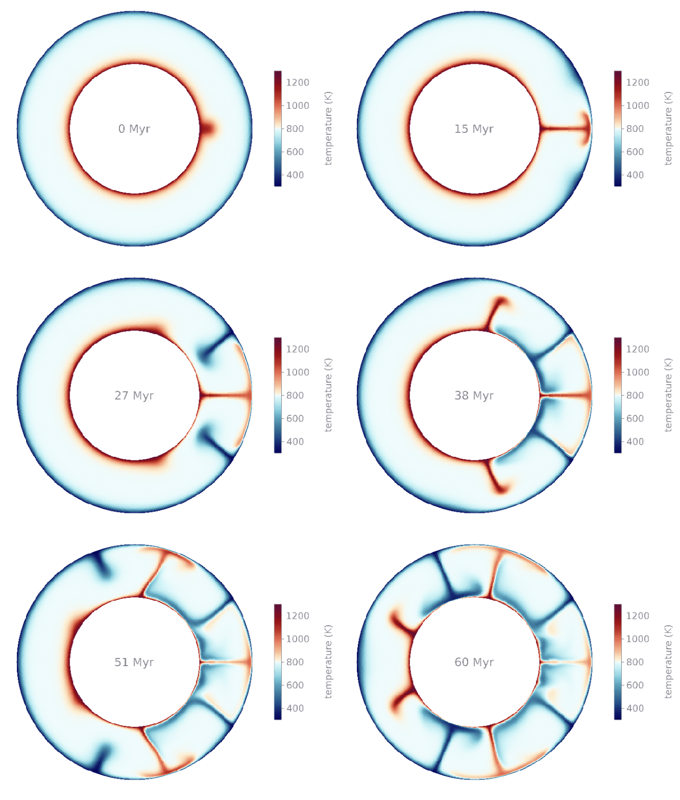
A short preview run of the driver as documented (isoviscous, Ra = 10⁶, 64 × 512, 1040 steps, 0 to 60 Myr of model time, a frame every 12 steps): temperature in the annulus, cold blue to hot red. The anomaly at azimuth 0 rises as a narrow conduit topped by a small head, reaches the cold boundary layer within about 15 Myr and spreads beneath it, while the cold boundary layer starts to drip down on both sides of the plume.

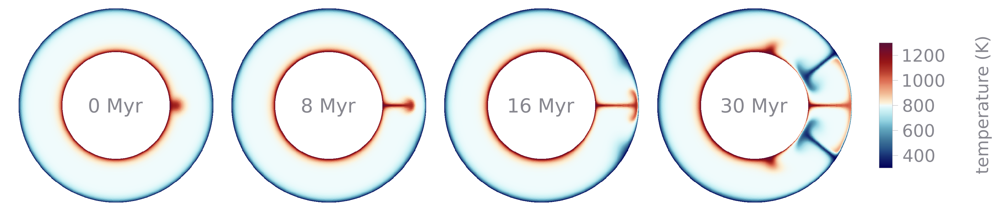
The same run at 0, 8, 16 and 30 Myr.

Running it

export GKSwstype=nul
julia --project=. -t 4 examples/annulus_plume_2d.jl 1e6 64          # isoviscous
julia --project=. -t 4 examples/annulus_plume_2d.jl 1e6 64 1e3      # Δη = 10³

Output goes to output/examples/plume_Ra1e+06_N64/ (or ..._dEta1e+03/). Open vtk/simulation.pvd in ParaView and colour by T_dev [K], the temperature minus its radial mean, to follow the plume.

What to expect

As an order-of-magnitude estimate, the Stokes velocity of the anomaly in units of $\kappa /D$ is about

$$V\sim \frac{\mathrm{Ra}}{3}\frac{\mathrm{\Delta }{T}_p}{\mathrm{\Delta }T}{\left(\frac{a}{D}\right)}^2=\frac{{10}^6}{3}\times 0.3\times 0.0225\approx 2\times {10}^3,$$

about 7 cm/yr, so the head should cross the 1000 km layer in a few tens of Myr and spend the rest of the 200 Myr spreading beneath the lid while the background boundary layers start to convect. A 2-D anomaly is a cylinder rather than a sphere, so its ascent is slower than this sphere-based estimate. With $\mathrm{\Delta }\eta ={10}^3$ the conduit should be visibly thinner than in the isoviscous case.

Smoke test

A quick check that the driver runs:

MILEVA_MAXSTEPS=6 julia --project=. -t 2 examples/annulus_plume_2d.jl 1e6 16 1e3

6 steps at 16 × 128 in 37 s of wall time; temperature and velocity finite, the largest temperature excess above the radial mean (268 K) sits in the seeded anomaly. At 64 × 512 (isoviscous) 40 steps took 0.56 s per step and 2.4 GB.