Material tables and viscosity profiles

MILEVA reads a mineral-physics property table and radial viscosity profiles (physics/material_tables.jl, data in data/steinberger/). The table sets the compressible reference state; the profiles give an Earth viscosity constrained by mineral physics and the geoid.

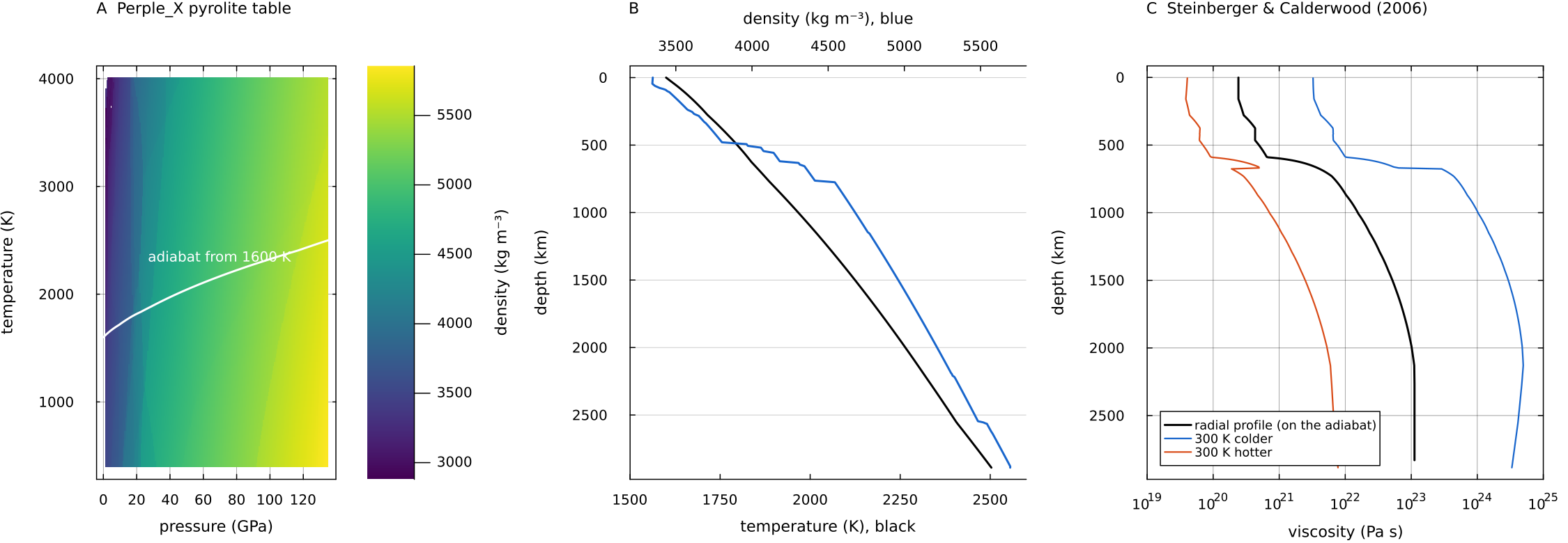
(A) Density in the Perple_X table of pyrolite, with the adiabat from 1600 K that the code integrates through it. (B) Temperature (black) and density (blue) along that adiabat; the steps are the olivine transitions near 410 and 520 km and the ringwoodite breakdown near 660 km. (C) The viscosity profile of Steinberger & Calderwood (2006), which is the viscosity on the adiabat, and the viscosity 300 K colder and hotter than it. Script: docs/scripts/fig_material_tables.jl.

Physical background

Why a convection model needs a reference state

Pressure in a planetary mantle rises from zero at the surface to more than a hundred gigapascals at the core-mantle boundary. Over that range rock is compressed and changes its mineral structure several times, so its density rises by roughly 70 per cent and its thermal expansivity falls by nearly a factor of three (from 3350 to 5700 kg/m³ and from $3.8\times {10}^{-5}$ to $1.4\times {10}^{-5}$ K⁻¹ along the adiabat of the pyrolite table below). None of this is captured by the Boussinesq approximation, which treats density as constant except in the buoyancy term. Compressible formulations such as the anelastic liquid approximation (Jarvis & McKenzie 1980) split every thermodynamic quantity into a depth-dependent reference part and a small departure from it. The reference part is a hydrostatic, adiabatic column, the state toward which vigorous convection homogenises the mantle interior. Convection is then described by the departures of temperature and density from that column. The reference state therefore sets how much buoyancy a given temperature anomaly produces at each depth, how fast rising and sinking rock cools and warms by decompression and compression, and how much heat a unit volume stores.

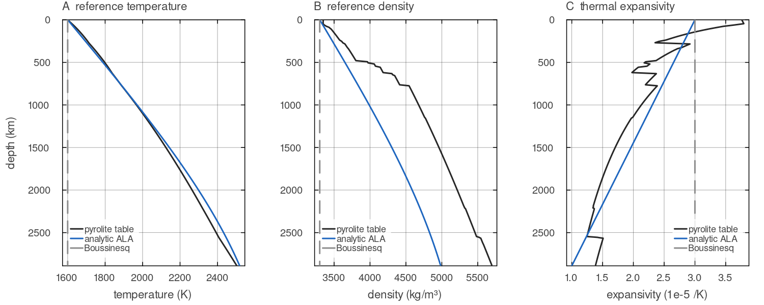
Three reference states on a 2890 km mantle at a 1600 K potential temperature. Black: table_adiabat through the shipped pyrolite table. Blue: the analytic ALA state of compressibility with the default SimConfig (linear expansivity from $3\times {10}^{-5}$ to $1\times {10}^{-5}$ K⁻¹). Grey: Boussinesq, constant cfg.rho0 and cfg.alpha. (A) The two adiabats differ by 40 K at most. (B) The table density rises from 3349 to 5695 kg/m³ in steps at the phase transitions, the analytic one smoothly to about 4980 kg/m³. (C) The table expansivity falls from $3.8\times {10}^{-5}$ to $1.4\times {10}^{-5}$ K⁻¹ with jumps where the mineralogy changes. Script: docs/scripts/fig_material_tables_sections.jl.

Why a thermodynamic table

A reference state can be written down analytically, for instance with a linear expansivity profile and a constant Grüneisen parameter, and MILEVA does this when no table is given (see Buoyancy and Heat sources). Such profiles are smooth and cannot carry the mineral phase transitions that dominate the transition zone. A thermodynamic table removes that restriction. A Gibbs free-energy minimisation code (Perple_X, Connolly 2005, 2009) takes a bulk composition and a self-consistent mineral database (Stixrude & Lithgow-Bertelloni 2005, 2011), finds the stable mineral assemblage at each pressure and temperature, and tabulates the aggregate density, expansivity and heat capacity on a regular grid. The table then contains the olivine to wadsleyite transition near 14 GPa, the wadsleyite to ringwoodite transition near 18 GPa and the breakdown of ringwoodite to bridgmanite and ferropericlase near 24 GPa, together with the gradual changes in the pyroxene and garnet components. Ita & King (1994) showed that the choice of equation of state can change the character of mantle flow. In their calculations an expansivity that decreases monotonically with depth and is unaffected by phase or temperature strongly enhanced layering at the 660 km transition, and the trend reversed once the pressure, temperature and phase dependence of the thermodynamic properties was included.

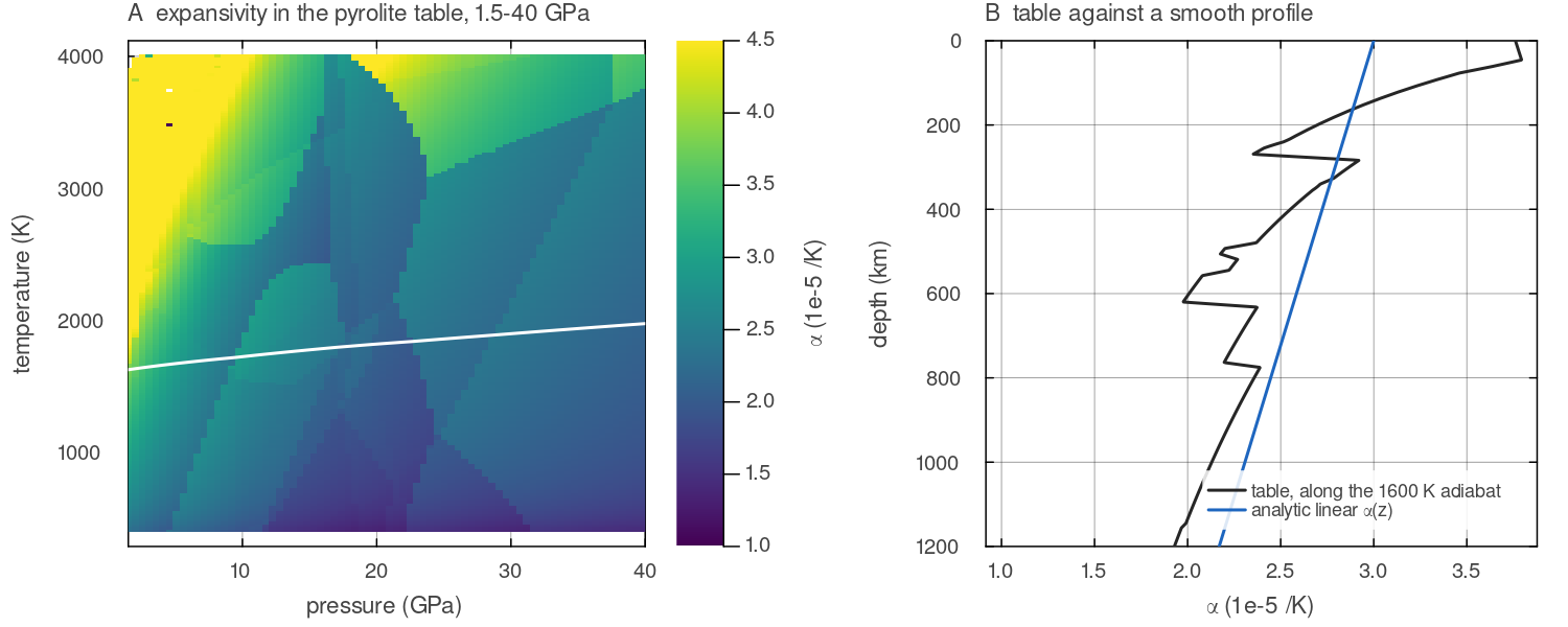
(A) Expansivity of the shipped table from 1.5 to 40 GPa, read by read_perplex_table, with the 1600 K adiabat of table_adiabat (white). The fields of the different mineral assemblages appear as patches with sharp edges. (B) The expansivity along that adiabat (black), with its steps near 14, 18 and 24 GPa (about 410, 520 and 660 km), against the linear profile of the analytic reference state (blue), which has none. Script: docs/scripts/fig_material_tables_sections.jl.

The adiabat and its scale

For a parcel that moves without exchanging heat, the first and second laws give the adiabatic temperature gradient

$${\left(\frac{dT}{dz}\right)}_S=\frac{\alpha gT}{c_p},$$

with $z$ depth, $\alpha$ the thermal expansivity, $g$ gravity and $c_p$ the isobaric heat capacity (Schubert, Turcotte & Olson 2001). Dividing it by $T$ defines the temperature scale height $H_T=c_p/(\alpha g)$, the depth over which the adiabatic temperature rises by a factor $e$, and the ratio of the mantle depth $D$ to $H_T$ is the dissipation number

$$Di=\frac{\alpha gD}{c_p},$$

the single parameter that measures how far a layer departs from Boussinesq behaviour (Jarvis & McKenzie 1980). When $Di\ll 1$ the adiabat is almost flat and the Boussinesq equations apply; when $Di$ is of order one, adiabatic heating, viscous dissipation and the depth dependence of the properties all matter. Integrating the gradient over the whole mantle gives $\ln (T_{\text{ad}}(D)/T_{\mathrm{pot}})={\int }_0^D\alpha g/c_{p}dz$, so the temperature ratio across the adiabat measures an effective dissipation number. For the pyrolite table used here, with $T_{\mathrm{pot}}$ = 1600 K and $g$ = 9.81 m/s², table_adiabat gives an adiabatic gradient of about 0.49 K/km at the top of the table, 0.30-0.36 K/km in the transition zone and 0.25-0.36 K/km in the lower mantle, the larger values near its top, and a temperature ratio of 2503/1600, an effective $Di$ of 0.45. The value from surface properties alone, $\alpha gD/c_p\approx 0.88$ with $\alpha =3.8\times {10}^{-5}$ K⁻¹ and the table's surface $c_p$ of about 1220 J/(kg K), is about twice as large, because the expansivity falls to about $1.4\times {10}^{-5}$ K⁻¹ near the core-mantle boundary. The difference shows why a depth-dependent expansivity matters.

The potential temperature $T_{\mathrm{pot}}$ is the temperature the mantle would have if brought adiabatically to the surface without melting. It labels an adiabat with one number. Estimates for Earth's present mantle are close to 1600 K, the value used in the Earth example. Katsura et al. (2010), for instance, give 1610 ± 35 K.

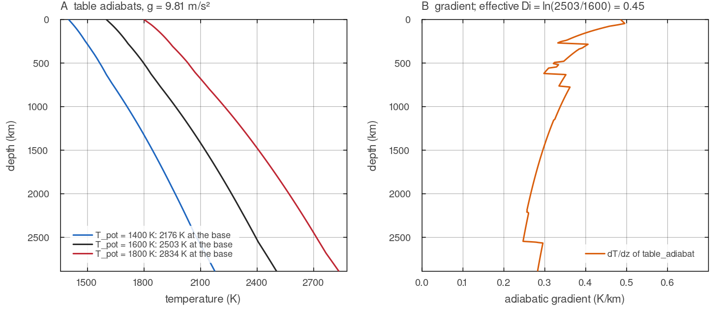
(A) table_adiabat from potential temperatures of 1400, 1600 and 1800 K with $g$ = 9.81 m/s², reaching 2176, 2503 and 2834 K at 2890 km. (B) The adiabatic gradient of the 1600 K adiabat, about 0.49 K/km at the top of the table and 0.25 to 0.36 K/km below the transition zone, with steps where the expansivity and heat capacity jump. The temperature ratio 2503/1600 gives an effective dissipation number of 0.45. Script: docs/scripts/fig_material_tables_sections.jl.

Radial viscosity structure

Viscosity in the mantle varies by many orders of magnitude, with temperature and with depth. The depth dependence along an adiabat is the part that a radial profile describes. It is constrained independently of laboratory creep laws by the long-wavelength geoid and by postglacial rebound. Hager (1984) showed that the positive correlation of the geoid with subducted slabs requires the effective viscosity to increase with depth by a factor of 30 or more, and joint inversions of convection-related and rebound data (Mitrovica & Forte

1. refine the shape of the increase. Steinberger & Calderwood (2006)

combined these surface observations with mineral physics. They computed the radial variation of viscosity in a few mantle layers with the aid of independent mineral physics results, which also gives the depth dependence of the temperature sensitivity, and determined the absolute viscosity of each layer by fitting the geoid, the Haskell average from postglacial rebound and the radial heat flux profile. Their profile without boundary layers, shipped with MILEVA, runs from $2.4\times {10}^{20}$ Pa s at the top to $1.1\times {10}^{23}$ Pa s in the lowermost mantle, a factor of about 460, with the steepest increase between about 590 and 740 km depth, around the 660 km transition. Their lateral profile $H/(nR)$ rises from about $1.8\times {10}^4$ K at the surface to $2.6\times {10}^4$ K above 660 km, jumps to $4.1\times {10}^4$ K below it and reaches $6.2\times {10}^4$ K at the core-mantle boundary, so the lower mantle is more sensitive to temperature than the upper mantle.

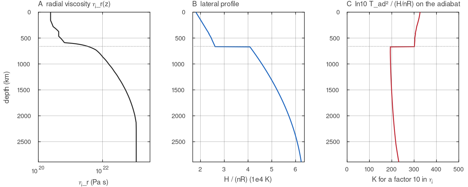
The two shipped Steinberger & Calderwood (2006) profiles as read_depth_profile and profile_value return them. (A) ${\eta }_r(z)$, $2.4\times {10}^{20}$ Pa s at the top rising to $1.1\times {10}^{23}$ Pa s, steepest between 590 and 740 km. (B) $H/(nR)$, with its jump at 660 km (dotted). (C) The temperature change that alters the viscosity tenfold on the 1600 K table adiabat, $\ln 10T_{\text{ad}}^2/(H/nR)$, about 300 to 330 K in the upper mantle and about 200 K in the lower mantle. Script: docs/scripts/fig_material_tables_sections.jl.

Earth and Venus values

The table is a function of pressure and temperature, not depth, so the same table can describe another planet once the adiabat is integrated with that planet's gravity. The values below come from table_adiabat applied to the shipped pyrolite table, with the Earth example parameters and with the Venus parameters quoted for the analytic adiabat in physics/compressibility.jl ($T_{\mathrm{pot}}$ = 1800 K, $g$ = 8.87 m/s², mantle depth 2942 km). They are outputs of this table and this integration, not independent estimates, and a Venus pyrolite is an assumption made only for the comparison.

	Earth (1600 K, 9.81 m/s²)	Venus (1800 K, 8.87 m/s²)
pressure at 660 km depth	24.2 GPa	21.3 GPa
depth at which the pressure reaches 24 GPa	about 657 km	about 733 km
temperature at 660 km depth	1849 K	2067 K
pressure at the base of the mantle	135.5 GPa (2890 km)	121.8 GPa (2942 km)
temperature at the base of the mantle	2503 K	2759 K
density at the base of the mantle	5695 kg/m³	5505 kg/m³

For Earth, PREM puts about 136 GPa at the core-mantle boundary (Dziewonski & Anderson 1981). The lower gravity of Venus means that a given pressure, and therefore a given phase transition, is reached about 11 per cent deeper than on Earth (24 GPa at 733 against 657 km). The radial viscosity profile, in contrast, is tabulated against depth and was fitted to Earth observations, so it does not transfer to another planet in the same way.

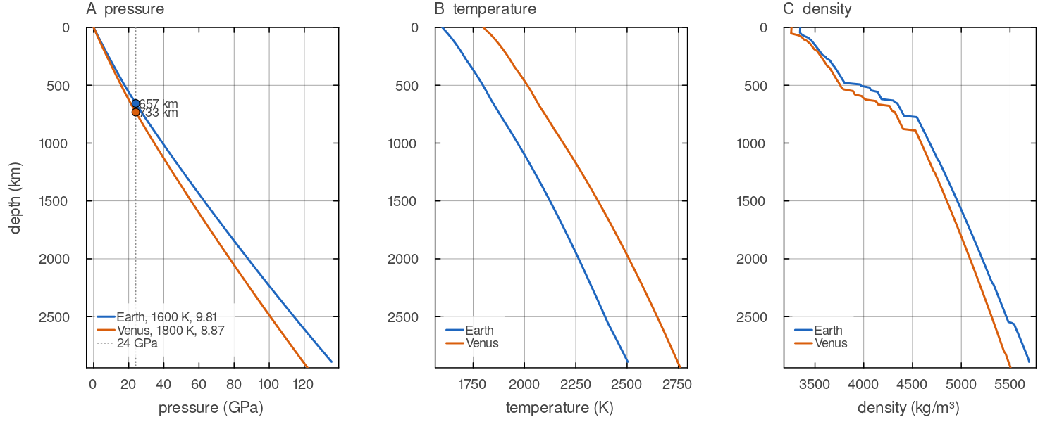
table_adiabat through the same pyrolite table with Earth parameters (1600 K, 9.81 m/s², 2890 km) and Venus parameters (1800 K, 8.87 m/s², 2942 km). (A) Pressure, with the depth at which 24 GPa is first reached in the 1 km steps of the integration, 657 km for Earth and 733 km for Venus. (B) Temperature. (C) Density, whose steps sit deeper on Venus because they are set by pressure. These are the values tabulated above. Script: docs/scripts/fig_material_tables_sections.jl.

The data

File	Content
pyr-ringwood88.txt	Perple_X table, 400-4000 K and 1.5-135 GPa on a 181 × 262 grid: density, thermal expansivity, heat capacity (and seismic velocities and enthalpy). Pyrolite of Ringwood (1988), database of Stixrude & Lithgow-Bertelloni (2011), computed with Perple_X (Connolly 2005).
radial-visc-simple.txt	viscosity against depth, Steinberger & Calderwood (2006) without boundary layers
temp-viscosity-prefactor.txt	$H/(nR)$ against depth, for the lateral temperature dependence

data/steinberger/README.md lists the files with their sources and licence.

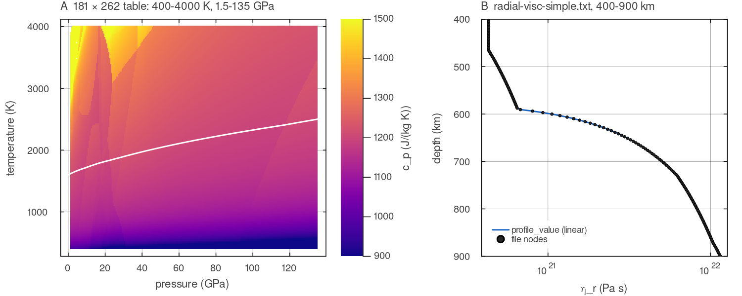
(A) The heat capacity column of pyr-ringwood88.txt over the full 181 × 262 grid, 400 to 4000 K and 1.5 to 135 GPa, with the 1600 K adiabat (white). (B) The nodes of radial-visc-simple.txt between 400 and 900 km and the linear interpolation profile_value applies between them. Script: docs/scripts/fig_material_tables_sections.jl.

Reference state from the table

The table only lists density, expansivity and heat capacity at fixed temperatures and pressures, so the code first reads that grid and then looks values up between its nodes by bilinear interpolation. To know which part of the table the mantle actually visits, it walks down from the surface in 1 km steps, letting temperature rise adiabatically and pressure build up with the weight of the rock above, and records density, expansivity and temperature along the way. That walk is the reference state. The viscosity then comes from a depth profile, multiplied by a factor that makes a cell stiffer when it is colder than the adiabat and softer when it is hotter, with that factor capped.

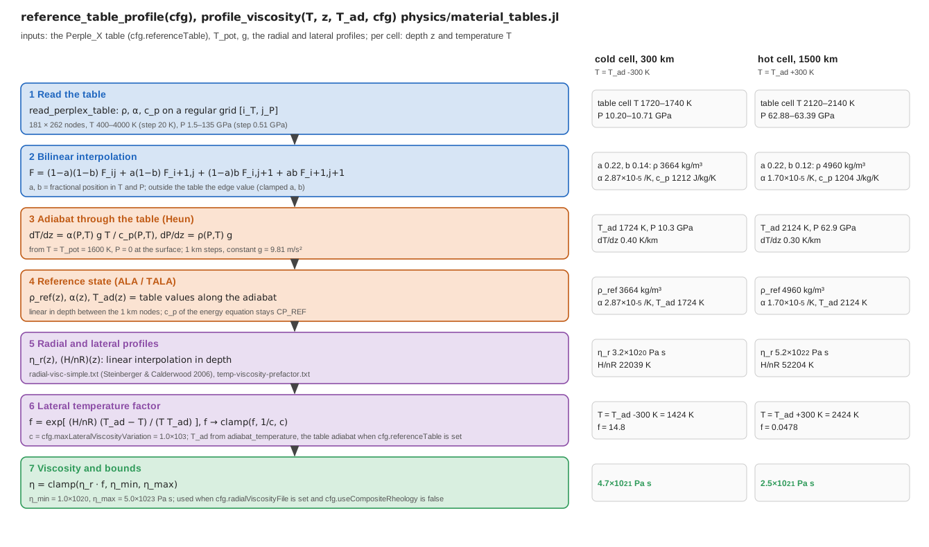
The computation in physics/material_tables.jl for the Earth setup (pyrolite table, $T_{\mathrm{pot}}$ = 1600 K, $g$ = 9.81 m/s², viscosity clamped to ${10}^{20}$-$5\times {10}^{23}$ Pa s). At 300 km the adiabat is at 1724 K and 10.3 GPa with ${\rho }_{\text{ref}}$ = 3664 kg/m³, and a cell 300 K colder gets a lateral factor of 14.8 on ${\eta }_r=3.2\times {10}^{20}$ Pa s, so $\eta =4.7\times {10}^{21}$ Pa s. At 1500 km the adiabat is at 2124 K and 62.9 GPa with ${\rho }_{\text{ref}}$ = 4960 kg/m³, and a cell 300 K hotter gets a factor of 0.048 on ${\eta }_r=5.2\times {10}^{22}$ Pa s, so $\eta =2.5\times {10}^{21}$ Pa s. Script: docs/scripts/fig_material_tables_pipeline.jl.

With cfg.referenceTable set and cfg.compressibilityMode = "ALA" or "TALA", the reference state is the adiabat of the table. From the surface, at $T=T_{\mathrm{pot}}$ (cfg.T_potential_ref) and $P=0$, the code integrates

$$\frac{dT}{dz}=\frac{\alpha (P,T)gT}{c_p(P,T)},\frac{dP}{dz}=\rho (P,T)g,$$

with bilinear interpolation in the table and constant gravity, and uses the temperature, density and expansivity along it as $T_{\text{ad}}(z)$, ${\rho }_{\text{ref}}(z)$ and $\alpha (z)$ everywhere the analytic reference state was used (initial condition, buoyancy, adiabatic heating). From 1600 K the adiabat reaches 2503 K and 135.5 GPa at 2890 km, against about 136 GPa at the core-mantle boundary of PREM. The heat capacity stays CP_REF.

Outside the table, at pressures below 1.5 GPa (the top 46 km of the 1600 K adiabat) or above 135 GPa, and outside 400-4000 K, the nearest edge value is used.

In these equations

Symbol	Meaning	Source in the code
$z$	depth below the surface, $R_{\text{out}}-r$	integration variable, 1 km steps
$T$	temperature on the adiabat	starts at cfg.T_potential_ref
$P$	lithostatic pressure, the weight of the column above	starts at 0
$\rho (P,T)$	density of the stable mineral assemblage	table column rho,kg/m3
$\alpha (P,T)$	volumetric thermal expansivity	table column alpha,1/K
$c_p(P,T)$	isobaric specific heat capacity	table column cp,J/K/kg
$g$	gravitational acceleration, constant with depth	cfg.g

The two equations are coupled, because the properties that set the temperature gradient depend on the pressure reached so far, and the density that sets the pressure gradient depends on the temperature. The code advances both together with Heun's method, a second-order predictor-corrector scheme that evaluates the right-hand sides at the start of a step and at an Euler estimate of its end and averages the two. The 1 km step is much finer than the table grid, 20 K in temperature and 0.51 GPa in pressure, which is about 15 km of depth near the top of the mantle and about 9 km near its base. A phase transition is therefore represented by a steep but continuous change of density across one table interval, and bilinear interpolation keeps the reference profiles continuous in depth.

The pressure is the lithostatic pressure of the reference column only. The dynamic pressure from the flow, which is smaller by orders of magnitude in the mantle interior, does not enter the lookup, and the properties are evaluated on the adiabat, not at the local temperature of each cell. The reference state is therefore one radial profile shared by every column of the model.

Viscosity from a radial profile

With cfg.radialViscosityFile set, the viscosity is

$$\eta ={\eta }_r(z)\exp [\frac{H}{nR}(z)\frac{T_{\text{ad}}-T}{T{T}_{\text{ad}}}],$$

where ${\eta }_r$ is the radial profile and $H/nR$ the lateral profile (cfg.lateralViscosityFile; without one the viscosity is radial only). The exponential factor is capped at cfg.maxLateralViscosityVariation (default 10³) either way, and the result is clamped to cfg.eta_min, cfg.eta_max. $T_{\text{ad}}$ is the model's reference adiabat (the table adiabat when cfg.referenceTable is set, the analytic one otherwise), so on the adiabat the viscosity is the profile itself. The composite rheology takes precedence, and the profile viscosity is used only while cfg.useCompositeRheology is false. This is the form of Steinberger & Calderwood (2006, Eq. 6) with the lateral average temperature replaced by the adiabat.

In this expression

Symbol	Meaning
${\eta }_r(z)$	viscosity on the adiabat at depth $z$, linearly interpolated in cfg.radialViscosityFile
$H$	activation enthalpy of the creep law
$n$	stress exponent of the creep law
$R$	gas constant
$(H/nR)(z)$	the depth profile read from cfg.lateralViscosityFile, in kelvin
$T$	temperature of the cell
$T_{\text{ad}}$	reference adiabat at the depth of the cell

The exponent is an Arrhenius ratio written relative to the adiabat, since

$$\frac{T_{\text{ad}}-T}{T{T}_{\text{ad}}}=\frac{1}{T}-\frac{1}{T_{\text{ad}}},$$

so the factor is $\exp [(H/nR)/T]/\exp [(H/nR)/T_{\text{ad}}]$, the ratio of the viscosity at the cell temperature to the viscosity on the adiabat for a creep law with activation enthalpy $H$. For power-law creep at a fixed strain rate the effective viscosity scales as $\exp [H/(nRT)]$, which is why $H$ appears divided by the stress exponent; for diffusion creep $n=1$. Laboratory values of $H$ and $n$ for olivine are compiled by Karato & Wu (1993) and Hirth & Kohlstedt (2003). Here the profile supplies the ratio directly, so neither $H$ nor $n$ is set separately.

Linearising the exponent about the adiabat gives the temperature sensitivity $d\ln \eta /dT\approx -(H/nR)/T_{\text{ad}}^2$. With the shipped profiles its magnitude is about $0.0074$ K⁻¹ at 300 km (a factor of ten for every 310 K) and about $0.0116$ K⁻¹ at 1500 km (a factor of ten for every 200 K). The two cells in the pipeline figure depart from this linear estimate, 14.8 rather than 9.2 and 0.048 rather than 0.031, because the exponent varies as $1/T$, which stiffens cold material more and softens hot material less than the linear rule. Cold material near the surface is stiffened strongly, but the cap of cfg.maxLateralViscosityVariation limits the effect. At 300 km the cap of ${10}^3$ is reached by a cell about 600 K colder than the adiabat, so the interior of a cold slab or of the lithosphere is at most a thousand times stiffer than the profile, and cfg.eta_max may bound it further. The radial profile has no boundary layers of its own. The thermal boundary layers at the top and bottom of the mantle appear in the viscosity only through this lateral factor, where the model temperature departs from the adiabat.

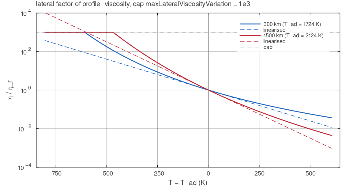
$\eta /{\eta }_r$ from profile_viscosity at 300 km ($T_{\text{ad}}$ = 1724 K) and 1500 km ($T_{\text{ad}}$ = 2124 K) along the 1600 K table adiabat, against the departure $T-T_{\text{ad}}$. Dashed lines are the linearised factor $\exp [-(H/nR)(T-T_{\text{ad}})/T_{\text{ad}}^2]$, dotted lines the default cap cfg.maxLateralViscosityVariation = ${10}^3$. Cold material is stiffened more than the linear rule predicts and reaches the cap at about 600 K below the adiabat at 300 km and about 470 K below it at 1500 km. Hot material is softened less than the linear rule predicts. Script: docs/scripts/fig_material_tables_sections.jl.

The Earth example uses both.

Assumptions and simplifications

• One bulk composition. The table is pyrolite. Basalt, depleted residue or any other composition tracked by the markers does not change the reference density, expansivity or adiabat. Compositional density contrasts enter through the buoyancy term (Buoyancy).

• A radial reference state. Density, expansivity and $T_{\text{ad}}$ depend on depth only. Thermal buoyancy uses ${\rho }_{\text{ref}}(z)\alpha (z)g$ times the lateral anomaly of $T-T_{\text{ad}}$, so the table enters the momentum equation through its values on the adiabat. The table density at each cell's own temperature is not used, and phase transitions in the table therefore shape the reference profile but do not by themselves produce the lateral density contrasts of a deflected phase boundary (Phase changes describes how MILEVA treats those).

• Constant gravity. The adiabat and the pressure are integrated with a single $g$. In PREM, gravity stays close to 10 m/s² through the mantle and rises to about 10.7 m/s² at the core-mantle boundary (Dziewonski & Anderson 1981). The effect on the reference pressure is small, 135.5 GPa at the base of the mantle against about 136 GPa in PREM.

• Heat capacity. The table $c_p$ is used only to integrate the adiabat. The energy equation keeps the constant CP_REF = 1250 J/(kg K); along the 1600 K adiabat the table gives 1190-1225 J/(kg K).

• Conductivity. The table carries no thermal conductivity, so conduction is unchanged by it (Governing equations).

• Edge values. Below 1.5 GPa the table has no data, and the shallowest 46 km of the Earth adiabat use the values at that edge.

• An Earth viscosity profile. ${\eta }_r(z)$ and $(H/nR)(z)$ are functions of depth fitted to Earth. Used for another planet they are a choice of the user, not a property of that planet.

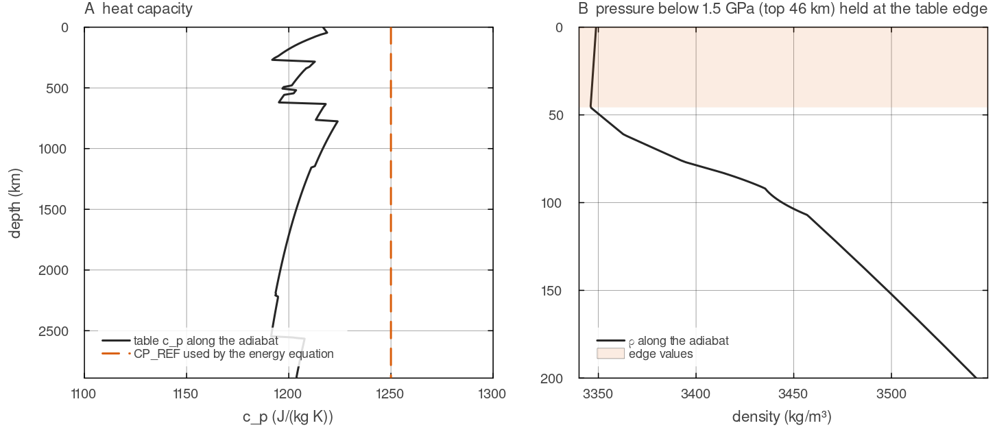
(A) The heat capacity of the pyrolite table along the 1600 K adiabat, 1190 to 1225 J/(kg K), against the constant CP_REF = 1250 J/(kg K) of the energy equation. (B) Density along the top 200 km of the adiabat. At pressures below 1.5 GPa, in the top 46 km, the lookup holds the pressure at the table edge, so the density there changes only with temperature. Script: docs/scripts/fig_material_tables_sections.jl.

Configuration

Field	Default	Meaning
cfg.referenceTable	""	Perple_X table for the ALA/TALA reference state; path absolute or relative to the repository
cfg.radialViscosityFile	""	viscosity against depth (km); replaces the simple viscosity path
cfg.lateralViscosityFile	""	$H/nR$ (K) against depth (km)
cfg.maxLateralViscosityVariation	1e3	cap on the lateral factor, either way

Where in the code

Topic	File	Function
Table reading and interpolation	physics/material_tables.jl	read_perplex_table, table_value
Profiles	physics/material_tables.jl	read_depth_profile, profile_value, profile_viscosity
Table adiabat	physics/material_tables.jl	table_adiabat, reference_table_profile
Use in the reference state	physics/compressibility.jl	adiabat_temperature, compressibility
Use in the time loop	main_SphCon.jl	viscosity step
Tests	tests/test_material_tables.jl	table grid, interpolation, adiabat, profile viscosity, reference state

References

Connolly, J. A. D. (2005), Earth Planet. Sci. Lett. 236, 524-541, doi:10.1016/j.epsl.2005.04.033. Steinberger, B. & Calderwood, A. R. (2006), Geophys. J. Int. 167, 1461-1481, doi:10.1111/j.1365-246X.2006.03131.x. Stixrude, L. & Lithgow-Bertelloni, C. (2011), Geophys. J. Int. 184, 1180-1213, doi:10.1111/j.1365-246X.2010.04890.x.

Connolly, J. A. D. (2009), The geodynamic equation of state: what and how, Geochem. Geophys. Geosyst. 10, doi:10.1029/2009GC002540. Dziewonski, A. M. & Anderson, D. L. (1981), Preliminary reference Earth model, Phys. Earth Planet. Inter. 25, 297-356, doi:10.1016/0031-9201(81)90046-7. Hager, B. H. (1984), Subducted slabs and the geoid: constraints on mantle rheology and flow, J. Geophys. Res. 89, 6003-6015, doi:10.1029/JB089iB07p06003. Hirth, G. & Kohlstedt, D. (2003), Rheology of the upper mantle and the mantle wedge: a view from the experimentalists, in Inside the Subduction Factory, Geophys. Monogr. 138, 83-105, doi:10.1029/138GM06. Ita, J. & King, S. D. (1994), Sensitivity of convection with an endothermic phase change to the form of governing equations, initial conditions, boundary conditions, and equation of state, J. Geophys. Res. 99, 15919-15938, doi:10.1029/94JB00852. Jarvis, G. T. & McKenzie, D. P. (1980), Convection in a compressible fluid with infinite Prandtl number, J. Fluid Mech. 96, 515-583, doi:10.1017/S002211208000225X. Karato, S. & Wu, P. (1993), Rheology of the upper mantle: a synthesis, Science 260, 771-778, doi:10.1126/science.260.5109.771. Katsura, T., Yoneda, A., Yamazaki, D., Yoshino, T. & Ito, E. (2010), Adiabatic temperature profile in the mantle, Phys. Earth Planet. Inter. 183, 212-218, doi:10.1016/j.pepi.2010.07.001. Mitrovica, J. X. & Forte, A. M. (2004), A new inference of mantle viscosity based upon joint inversion of convection and glacial isostatic adjustment data, Earth Planet. Sci. Lett. 225, 177-189, doi:10.1016/j.epsl.2004.06.005. Schubert, G., Turcotte, D. L. & Olson, P. (2001), Mantle Convection in the Earth and Planets, Cambridge University Press, doi:10.1017/CBO9780511612879. Stixrude, L. & Lithgow-Bertelloni, C. (2005), Thermodynamics of mantle minerals I. Physical properties, Geophys. J. Int. 162, 610-632, doi:10.1111/j.1365-246X.2005.02642.x.

Further reading

• Schubert, Turcotte & Olson (2001), a textbook treatment of the adiabat, the Grüneisen parameter, the dissipation number and compressible convection.

• Jarvis & McKenzie (1980), the derivation of the anelastic liquid equations and of the reference state they rest on.

• Connolly (2009), how phase-equilibrium calculations provide equation-of-state tables for geodynamic models.

• Stixrude & Lithgow-Bertelloni (2005, 2011), the mineral database behind the shipped table.

• Steinberger & Calderwood (2006), the construction of the radial and lateral viscosity profiles used here.

• Steinberger, B., Werner, S. C. & Torsvik, T. H. (2010), Deep versus shallow origin of gravity anomalies, topography and volcanism on Earth, Venus and Mars, Icarus 207, 564-577, doi:10.1016/j.icarus.2009.12.025, for geoid and topography modelling with radial viscosity structure on Earth, Venus and Mars.