Energy budget and heat-flow diagnostics

A model that leaks heat can still produce plausible temperatures, velocities and Nusselt numbers. MILEVA therefore logs a discrete energy budget with every row of diagnostics.csv, built from the same fluxes and the same time weighting the solver uses, so its residual tests conservation rather than sampling. This page defines the budget columns and the Nusselt numbers.

The budget

The thermal energy of the domain is

$$E_{\text{th}}={\rho }_0{c}_p\sum _c{T}_c{V}_c,$$

with $V_c$ the cell measure of the run's geometry (cell_areas and cell_volumes), scaled to physical walls: in the spherical annulus each column stands for $1/N_t$ of a full sphere, so a wall has area $4\pi r^2$; in the cylinder the budget is per unit length, $2\pi r$. The diagnostics use $c_p=1250{\text{J kg}}^{-1}{\text{K}}^{-1}$, the value the diffusion solver uses.

Each step the main loop accumulates the energy supplied,

$$E_{\text{bnd}}+=\mathrm{\Delta }t(P_{\text{in}}-P_{\text{out}}+P_{\text{int}}),P=\theta P(T^{n+1})+(1-\theta )P(T^n),$$

where $P_{\text{in}}$ and $P_{\text{out}}$ are the core-mantle boundary and surface powers from boundary_power(Tg, grid, cfg), $\theta$ is the diffusion solver's own implicitness (cfg.implicitTheta when useImplicitTemp, else 0), and $P_{\text{int}}$ is the internal heating the solver actually applied in that call (internal_power_last(): radiogenic, latent, heat pipe and any uniform source). Between two CSV rows the residual is

$$\mathtt{\text{budget\_resid}}=\frac{{\displaystyle \frac{\mathrm{\Delta }{E}_{\text{th}}}{\mathrm{\Delta }{t}_{\text{row}}}}-{\displaystyle \frac{\mathrm{\Delta }{E}_{\text{bnd}}}{\mathrm{\Delta }{t}_{\text{row}}}}}{⟨max(|P_{\text{out}}|,|P_{\text{int}}|){⟩}_{\text{row}}},$$

normalised by the larger of the surface power and the internal power, taken every step and averaged over the interval (E_out_cum in main_SphCon.jl), so an internally heated run with a small surface flux still has a meaningful denominator. A conservative scheme gives zero whatever the heating mode.

Column	Meaning
E_th_J	$E_{\text{th}}$ at this row
dEdt_W	mean $d{E}_{\text{th}}/dt$ since the previous row
P_supplied_W	mean supplied power since the previous row (boundaries plus internal heating)
budget_resid	the residual above; the log line prints it as bud=
E_core_J, E_cmb_cum_J, budget_resid_joint	the same budget for core plus mantle, when the 2-D core cools (cmbHeatfluxMode = "parameterized"); NaN otherwise

E_cmb_cum_J restarts at zero when a run is resumed; difference it, never read it as an absolute value.

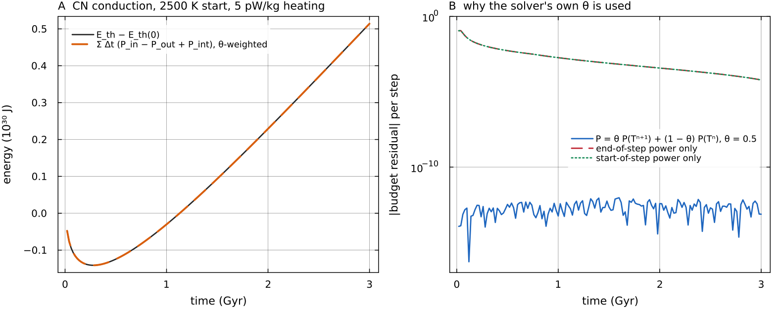
Conduction in the default shell ($64\times 8$, ALA) from a uniform 2500 K interior with 5 pW/kg of internal heating, advanced by diffuse_temperature with Crank-Nicolson steps of 20 Myr. Left: the change of thermal_energy and the energy supplied, accumulated from boundary_power and internal_power_last with the solver's $\theta =0.5$; the two curves coincide. Right: the per-step residual of the budget formula. With the $\theta$-weighted wall power it is about ${10}^{-12}$; using only the end-of-step or only the start-of-step power leaves a residual of ${10}^{-2}$ to ${10}^{-1}$ that decays only as the transient does, which is a timing error of the bookkeeping, not a leak. Script: docs/scripts/fig_numerics_energy_budget_sections.jl.

Wall fluxes and Nusselt numbers

The wall temperatures are held at the faces $R_{\text{in}}$ and $R_{\text{out}}$ through a half-cell ghost (see Temperature transport), and the reported fluxes are exactly the ones the diffusion operator uses:

$$q_{\text{top}}=-k\frac{T_{\text{surf}}-T_{N_r}}{R_{\text{out}}-r_{N_r}},q_{\text{bot}}=-k\frac{T_1-T_{\text{cmb}}}{r_1-R_{\text{in}}},$$

averaged over the wall cells. The Nusselt numbers divide them by the conductive flux of the same geometry. Steady conduction has $r^{m}kdT/dr$ constant, so

$$q_{\text{cond}}(r)=\frac{C}{r^m},C=\frac{T_{\text{cmb}}-T_{\text{surf}}}{{\displaystyle {\int }_{R_{\text{in}}}^{R_{\text{out}}}\frac{dr}{r^m\kappa (r)}}},{\text{Nu}}_{\text{top}}=\left|\frac{q_{\text{top}}}{q_{\text{cond}}(R_{\text{out}})}\right|,{\text{Nu}}_{\text{bot}}=\left|\frac{q_{\text{bot}}}{q_{\text{cond}}(R_{\text{in}})}\right|,$$

(compute_diagnostics in utils/compute_diagnostics.jl, conductive_baseline_C in physics/compressibility.jl). Flux and baseline use the diffusivity the model transports with, which matters under ALA where $\kappa$ rises toward the core. In 3-D the baseline is $C/r^2$.

Two internal checks follow. On a conducting field Nu = 1, and at a steady state with basal heating Nu${}_{\text{top}}$ = Nu${}_{\text{bot}}$, because the same power crosses every shell. Neither depends on any published reference value. tests/test_nusselt_conduction.jl asserts both forms on the solver's own conducting steady state: Nu converges to 1 (error ${10}^{-3}$ falling to $5\times {10}^{-5}$ with refinement) and a one-step budget residual is $2\times {10}^{-15}$.

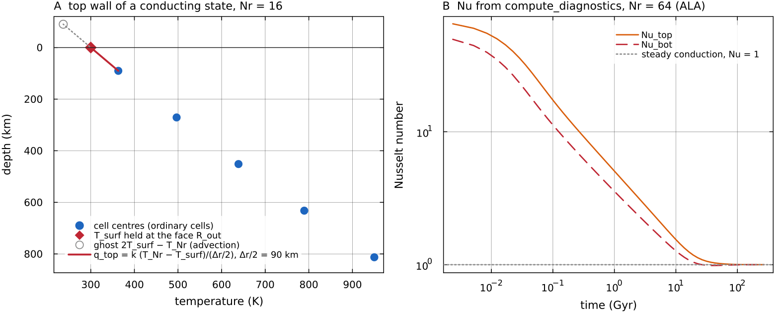
Left: the top of a conducting steady state on a 16-cell column. The surface temperature is held at the face $R_{\text{out}}$, half a cell above the top cell centre, and the reported flux is the slope of the red segment, $k(T_{N_r}-T_{\text{surf}})/(\frac{1}{2}\mathrm{\Delta }r)$; the open circle is the reflected ghost used by the advection schemes. Right: Nu_top and Nu_bot from compute_diagnostics while a uniform 2000 K interior relaxes to conduction ($N_r=64$, ALA, backward Euler). Both fall to 1 (1.000014 and 0.999950 at the end) and agree with each other once the state is steady, as the two internal checks require. Script: docs/scripts/fig_numerics_energy_budget_sections.jl.

Measured residuals

tests/test_marker_energy.jl pins the marker step: energy delivered equals energy computed to $3\times {10}^{-15}$ in 2-D and $5\times {10}^{-11}$ in 3-D.

Residuals on the Hernlund & Tackley (2008) spherical-annulus verification runs (window means; the benchmark comparison itself is documented elsewhere):

Case	$N_r$	budget_resid
Ra = ${10}^4$, isoviscous	128	$-0.0004$
Ra = ${10}^5$, isoviscous	128	$-0.001$
Ra = ${10}^5$, viscosity contrast ${10}^6$	64	$+0.0015$
Ra = ${10}^5$, isoviscous, start-up transient	32	$+0.003$ per 500-step window
Ra = ${10}^5$, temperature on the grid with TVD	64	$+0.011$

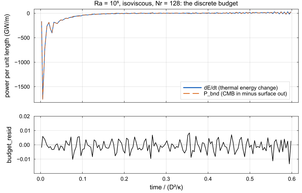
diagnostics.csv of the Ra = ${10}^5$ isoviscous verification run at $N_r=128$. Top: the change of thermal energy and the net wall power, which lie on top of each other through the start-up transient and the time-dependent state. Bottom: budget_resid, scattered between about −0.01 and +0.01.

Sources of small residuals

• Reseeding. A cell that has emptied completely gets markers with temperatures interpolated from the grid; that is the one non-conservative marker operation (see Markers).

• The delivery cap. Energy withheld by cfg.deliveryScaleMax at sparsely populated nodes appears in the residual.

• Temperature clamps. The bounds applied after diffusion and after the hand-back remove energy only when they bind, which on a well-resolved run they do not.

• Grid TVD advection gives a slightly larger residual, as the table shows.

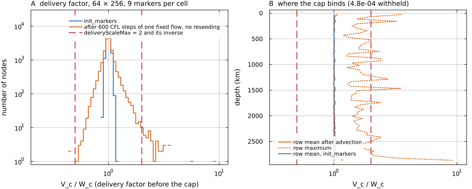
The delivery cap as a residual source. Left: the factor $V_c/W_c$ that measure-scaled delivery applies at each node of a $64\times 256$ Boussinesq annulus, for the markers of init_markers (9 per cell) and after 600 CFL steps through one fixed two-cell Stokes flow with no reseeding. Advection widens the distribution and pushes a few nodes past deliveryScaleMax = 2. Right: row means and row maxima with depth; the cap binds mostly in single cells and in the bottom wall row. For a uniform increment the cap withholds $4.8\times {10}^{-4}$ of the energy in this state, which then appears in budget_resid. Script: docs/scripts/fig_numerics_energy_budget_sections.jl.

3-D

In 3-D the row is computed on the Yin patch only (E_th "this patch only" in diagnostics_row), with the patch's own wall areas. Because the Yin patch overlaps Yang (see Markers), the 3-D budget_resid is a diagnostic of that patch rather than a global budget.

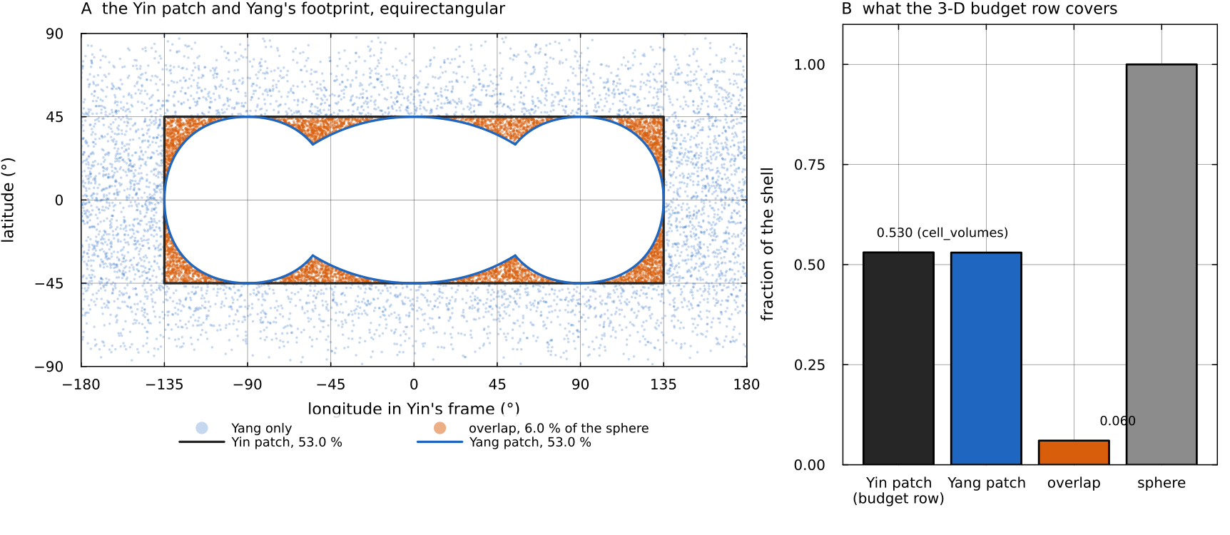
Left: the Yin patch (black rectangle) and the boundary of the Yang patch mapped into Yin's frame with yy_yang_to_yin, sampled with random points on the sphere. Each patch covers 53.0 % of the sphere and they overlap on 6.0 % (orange). Right: the 3-D budget row integrates the Yin patch only; cell_volumes gives 0.530 of the shell at $N_{\theta }=12$, so the row covers about half the mantle and includes the overlap band that Yang also holds. Script: docs/scripts/fig_numerics_energy_budget_sections.jl.

Where in the code

Topic	File	Function
Budget accumulation	main_SphCon.jl	step (14), E_bnd_cum, E_out_cum, E_cmb_cum
Wall powers	utils/diagnostics_csv.jl	boundary_power
CSV row and residual	utils/diagnostics_csv.jl	diagnostics_row, _diag_row_common
Applied internal power	solvers/diffuse_temperature.jl	internal_power_last
Nusselt numbers	utils/compute_diagnostics.jl	compute_diagnostics
Conductive baseline	physics/compressibility.jl	conductive_baseline_C
Tests	tests/	test_nusselt_conduction.jl, test_marker_energy.jl, test_conduction_conservation.jl, test_energy_consistency.jl