Buoyancy and composition

The body force in the momentum equation is radial, $\mathbf{b}=b\hat{\mathbf{r}}$, built each step by compute_buoyancy (physics/compute_buoyancy.jl) from a density perturbation:

$$b=-g\delta \rho ,\delta \rho =\delta {\rho }_T+\delta {\rho }_{\text{phase}}+\delta {\rho }_{\text{Clap}}+\delta {\rho }_C,$$

positive outward, so light material rises. Gravity $g$ = cfg.g is uniform in radius. Every thermal and phase term is a lateral anomaly: its horizontal mean at each radius is removed, because a purely radial body force is balanced by a pressure gradient and drives no flow. The hydrostatic reference therefore never enters the solve.

The force is built one density contribution at a time and added up at the end. Temperature comes first, and a cell hotter than the rest of its row is lighter. Phase transitions come next, and they matter only where heat or cold has moved a boundary up or down. Composition follows. Depleted residue is lighter, while pile material and basalt that has turned to eclogite are heavier. The sum of these density differences, multiplied by gravity, is the push the flow solver sees.

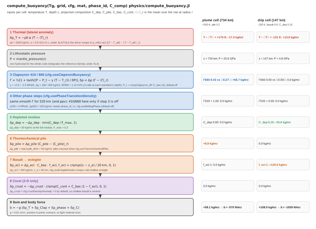
The stages of compute_buoyancy (2-D) on a strip of eight columns, with Clapeyron buoyancy switched on (cfg.useClaperonBuoyancy = true) and cfg.Nr = 128. Two example cells sit in the first column; the other seven are the reference adiabat with no composition, so each lateral anomaly is taken against a row mean that includes the example cell (a 200 K excess becomes a 175 K anomaly). The plume cell (734 km, +200 K, pile fraction 0.2) is made heavier, not lighter, because the negative Clapeyron slope lifts the 660 km analogue in hot material. The cell is therefore already in the dense phase while its row is not, which adds +66.7 kg/m³ against a thermal −17.3 kg/m³, and the pile adds +8.8 kg/m³, giving +58.1 kg/m³ and b = −570 N/m³. The drip cell (147 km, −150 K, basalt 0.6, depletion 0.15) gets +13.0 kg/m³ from its temperature, +120.0 kg/m³ from eclogite and −25.0 kg/m³ from depletion, giving +108.0 kg/m³ and b = −1059 N/m³. The thermal values are the Boussinesq form that compute_buoyancy returns; under the default cfg.compressibilityMode = "ALA" the driver replaces that term with the reference-state form given below. Every value is checked against compute_buoyancy itself. Script: docs/scripts/fig_buoyancy_pipeline.jl.

Physical background

What drives the flow

Mantle convection is driven by density differences in a gravitational field. A parcel that is lighter than the material beside it at the same depth is pushed upward, a heavier one sinks, and the speed at which either moves is set by how strongly the surrounding rock resists being sheared. The mantle is so viscous that inertia plays no part. Its Prandtl number, the ratio of momentum diffusivity $\eta /\rho$ to thermal diffusivity $\kappa$, is of order ${10}^{23}$ or larger (Schubert, Turcotte & Olson 2001). The momentum equation therefore reduces to an instantaneous balance between the body force, the viscous stresses and the pressure gradient (Stokes flow). Whatever density field exists at a given moment fixes the velocity field at that moment, and the body force $\mathbf{b}$ built on this page is the only source of motion in that balance. Every other piece of physics in MILEVA (heating, melting, rheology) changes the flow by changing either this density field or the viscosity that resists it.

A useful scale for the speed this produces is Stokes' result for a rigid sphere of radius $a$ and density contrast $\mathrm{\Delta }\rho$ moving through a fluid of viscosity $\eta$ (Turcotte & Schubert 2014),

$$v_{\text{Stokes}}=\frac{2}{9}\frac{\mathrm{\Delta }\rho g{a}^2}{\eta }.$$

With $\mathrm{\Delta }\rho =50$ kg m${}^{-3}$, Venus gravity $g=8.87$ m s${}^{-2}$ (NASA Venus Fact Sheet), $a=100$ km and $\eta ={10}^{21}$ Pa s this gives about 3 cm per year. The velocity grows with the square of the size of the anomaly and falls inversely with viscosity, which is why both the density contrast and the viscosity field must be right before a model velocity means anything.

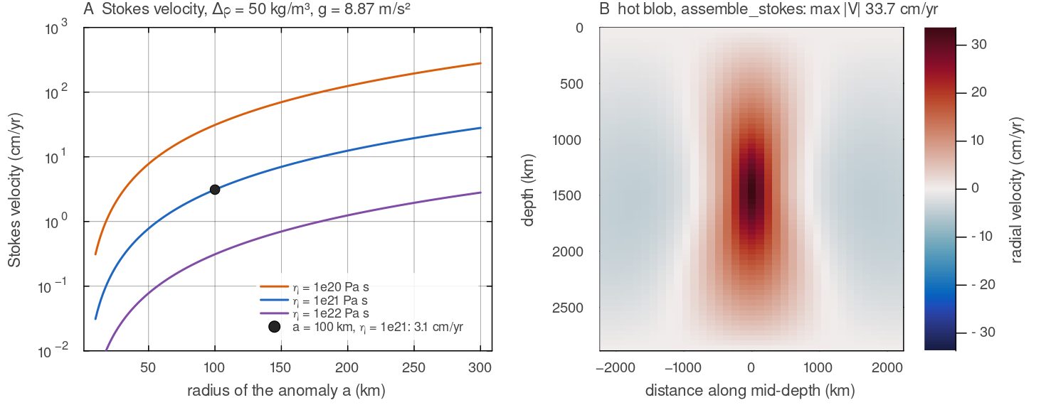
(A) Stokes' sphere velocity $\frac{2}{9}\mathrm{\Delta }\rho g{a}^2/\eta$ for $\mathrm{\Delta }\rho$ = 50 kg/m³ and Venus gravity; the dot is the 3 cm/yr example of the text. (B) The same physics in MILEVA: a blob 500 K hotter than a 1600 K mantle (Gaussian, 150 km standard deviation, at mid-depth) gives a body force through compute_buoyancy, and one direct solve of assemble_stokes with $\eta ={10}^{21}$ Pa s returns the radial velocity shown, rising through the blob and returning on both sides, with a peak speed of 33.7 cm/yr. Default shell, Boussinesq, 64 × 256 cells (an operator illustration). Script: docs/scripts/fig_buoyancy_sections.jl.

Where density differences come from

Three processes change the density of mantle rock at a given depth.

• Temperature. Rock expands when heated. The fractional density change per kelvin is the thermal expansivity $\alpha$, about $3\times {10}^{-5}$ K${}^{-1}$ in the upper mantle and decreasing with depth by a factor of several towards the core-mantle boundary (Schubert, Turcotte & Olson 2001). A plume 100 K hotter than its surroundings is therefore lighter by roughly 0.3 per cent, about 10 kg m${}^{-3}$. Heating from below and within, and cooling from above, continually create thermal anomalies, and this is what keeps convection going.

• Composition. Rocks of different chemistry have different densities at the same pressure and temperature. Partial melting preferentially removes iron and the garnet-forming components into the melt, so the solid residue (harzburgite) is lighter than fertile peridotite. Jordan (1978) proposed that this compositional buoyancy offsets the negative thermal buoyancy of cold, depleted continental roots, so that they neither sink nor rise. The melt, once it has frozen to basalt and been carried below a few tens of kilometres, transforms to eclogite, which is denser than the surrounding peridotite through most of the upper mantle (Irifune & Ringwood 1993). Material of distinct bulk composition at the base of the mantle, the thermochemical piles, is usually taken to be denser than the mantle above it.

• Phase changes. The minerals of the mantle transform to denser structures as pressure rises, producing density steps of several per cent near 410 and 660 km depth on Earth (Dziewonski & Anderson 1981). A step that sits at the same depth everywhere drives no flow. A step that a hot or cold anomaly has displaced up or down does, because over the displacement the anomaly is in a different phase from its surroundings (Christensen & Yuen 1985). The sign of this effect depends on the slope of the phase boundary in pressure and temperature and is set out on the Phase changes page.

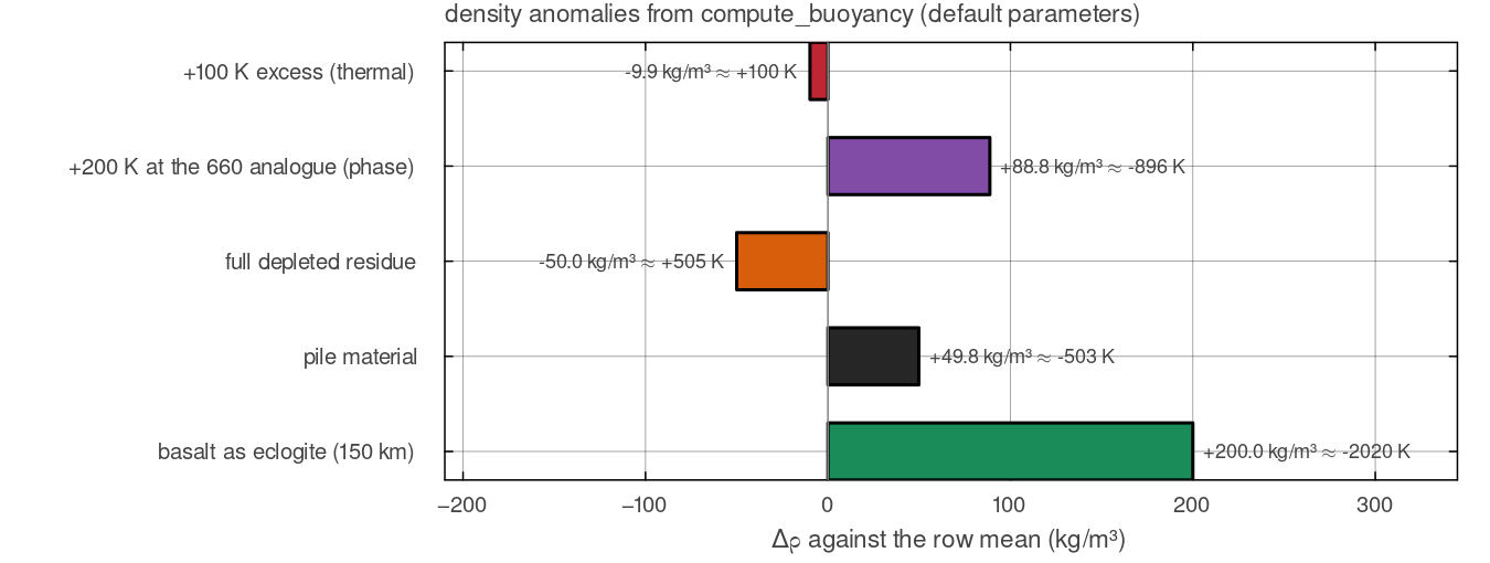
One column of each kind against an otherwise uniform row, from the parts that compute_buoyancy reports. The bars are a 100 K excess at 300 km ($-9.9$ kg/m³), the largest anomaly of the 660 km analogue in a column 200 K hotter than the adiabat (+88.8 kg/m³, Clapeyron buoyancy on), a full depleted residue ($-50$), pile material (+49.8, the row mean removed), and basalt that has become eclogite at 150 km (+200). The labels give the temperature difference $-\mathrm{\Delta }\rho /({\rho }_0\alpha )$ that would produce the same density. Default shell, 128 × 256 cells. Script: docs/scripts/fig_buoyancy_sections.jl.

Only lateral differences matter

A density that changes with radius only, the same at every point of a spherical shell, produces a body force $b(r)\hat{\mathbf{r}}$ that is the gradient of a potential, $\mathrm{\nabla }\mathrm{\Phi }$ with $\mathrm{\Phi }(r)=\int bdr$. A change in pressure balances it exactly and no motion results. This is the hydrostatic state, and it is why the absolute density of the mantle, rising from about 3400 to 5600 kg m${}^{-3}$ between the top and the bottom of Earth's mantle (Dziewonski & Anderson 1981), never needs to enter the momentum equation. What drives convection is the difference between a point and the average of its radius. MILEVA uses this freedom in two ways. The thermal, phase and pile terms are written as lateral anomalies from the outset, which keeps the numbers the solver handles small and centred on zero. The depletion, eclogite and crust terms are not mean-removed; their radial mean changes only the pressure and leaves the velocity unchanged.

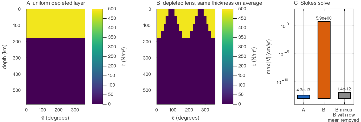
(A) A fully depleted layer 200 km thick at every angle and (B) a lens whose thickness varies as $100+100\cos 2\theta$ km, both as body forces from compute_buoyancy. (C) Largest speed of a direct assemble_stokes solve with $\eta ={10}^{21}$ Pa s. The uniform layer drives $4\times {10}^{-13}$ cm/yr, round-off, while the lens drives 5.9 cm/yr. Removing the row mean from the lens's force changes the velocity by $1.4\times {10}^{-12}$ cm/yr, so only the lateral part of a force moves the mantle. Default shell, 64 × 256 cells, Boussinesq. Script: docs/scripts/fig_buoyancy_sections.jl.

Measuring buoyancy without units

Three dimensionless numbers summarise how strongly each kind of density difference competes with the others.

number	definition	meaning
thermal Rayleigh number	$Ra={\rho }_{0}g\alpha \mathrm{\Delta }T{D}^3/(\kappa \eta )$	vigour of thermal convection across a layer of depth $D$ and temperature contrast $\mathrm{\Delta }T$; see Governing equations
buoyancy number	$B=\mathrm{\Delta }{\rho }_C/({\rho }_0\alpha \mathrm{\Delta }T)$	compositional density contrast measured against the thermal one
phase buoyancy parameter	$\mathcal{P}=\gamma \mathrm{\Delta }{\rho }_k/(\alpha {\rho }_0^{2}gD)$	effect of a phase transition with Clapeyron slope $\gamma$ and density jump $\mathrm{\Delta }{\rho }_k$, relative to thermal buoyancy (Christensen & Yuen 1985)

The buoyancy number decides whether a compositionally distinct layer stays where it is or is stirred into the convecting mantle; laboratory experiments show a transition from a stable stratified layer to one that rises and sinks in domes as $B$ falls (Davaille 1999). A negative $\mathcal{P}$ belongs to an endothermic transition that resists flow across it, and the more negative it is, the closer the mantle comes to convecting in two separate layers (Christensen & Yuen 1985). With the default parameters of MILEVA (${\rho }_0=3300$ kg m${}^{-3}$, $\alpha =3\times {10}^{-5}$ K${}^{-1}$, $g=9.81$ m s${}^{-2}$, $D=2890$ km, and the 660 km analogue at $\gamma =-2.5$ MPa K${}^{-1}$, $\mathrm{\Delta }\rho =400$ kg m${}^{-3}$), $\mathcal{P}\approx -0.11$ for the 660 km analogue and $+0.05$ for the 410 km one.

A simple way to compare the terms on this page is the temperature difference that would give the same density difference, $\mathrm{\Delta }\rho /({\rho }_0\alpha )$. With the defaults, ${\rho }_0\alpha =0.099$ kg m${}^{-3}$ K${}^{-1}$, so the 50 kg m${}^{-3}$ of a full depleted residue is worth about 500 K of heating and the 200 kg m${}^{-3}$ of eclogite about 2000 K of cooling. Compositional anomalies are rarely as concentrated as these end members, but where they are, they outweigh the thermal ones.

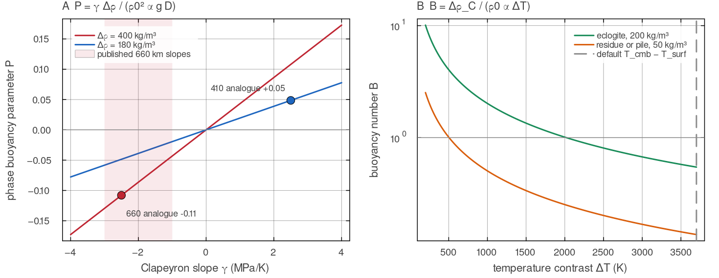
(A) $\mathcal{P}$ against Clapeyron slope for the density jumps of the 410 and 660 km analogues (mat.drho_410, mat.drho_660), with the model defaults marked ($+0.05$ and $-0.11$) and the range of published 660 km slopes shaded. (B) The buoyancy number of eclogite (200 kg/m³) and of residue or pile material (50 kg/m³) against the temperature contrast; the dashed line is the default contrast T_cmb - T_surf = 3700 K, at which $B$ is 0.55 and 0.14. Values from SimConfig, MaterialProperties and TemperatureConditions defaults. Script: docs/scripts/fig_buoyancy_sections.jl.

Thermal buoyancy

Under cfg.compressibilityMode = "Boussinesq":

$$\delta {\rho }_T=-{\rho }_0\alpha (T-⟨T{⟩}_r),$$

with $⟨\cdot {⟩}_r$ the mean over all cells at radius $r$ (over $\theta$ in 2-D, over $\theta$ and $\varphi$ on the Yin patch in 3-D).

where

$${\rho }_0$$

= cfg.rho0 (default 3300 kg m${}^{-3}$) is the reference density,

• $$\alpha$$

  = cfg.alpha (default $3\times {10}^{-5}$ K${}^{-1}$) is the thermal expansivity, constant in this mode,

• $$T$$

  is the cell temperature, the grid field Tg, and

• $$T-⟨T{⟩}_r$$

  is its excess over the mean of its row.

The minus sign makes a hot cell light: $\delta {\rho }_T<0$, so $b=-g\delta {\rho }_T>0$ and the force points outward. With the defaults a 100 K excess gives $\delta {\rho }_T=-9.9$ kg m${}^{-3}$ and $b\approx +97$ N m${}^{-3}$. This is the Boussinesq approximation. Density differences are kept only where they are multiplied by gravity, and everywhere else the fluid is treated as having the constant density ${\rho }_0$ (Schubert, Turcotte & Olson 2001).

Under ALA and TALA the driver (main_SphCon.jl, step 4) replaces this term with the reference-state form

$$b_T={\rho }_{\text{ref}}(r)\alpha (r)g[(T-T_{\text{ad}})-⟨T-T_{\text{ad}}{⟩}_r],$$

using ${\rho }_{\text{ref}}$, $\alpha (r)$ and $T_{\text{ad}}$ from compressibility (physics/compressibility.jl), and keeps the phase and compositional terms of compute_buoyancy. Since $T_{\text{ad}}$ depends on radius only, this is the lateral temperature anomaly weighted by the local density and expansivity.

The anelastic liquid approximation (Jarvis & McKenzie 1980) lets the reference density and expansivity vary with depth along an adiabat while still filtering out sound waves. For buoyancy its main consequence is physical rather than formal. A given temperature anomaly is less buoyant at depth, because $\alpha (r)$ falls towards the core-mantle boundary, and slightly more buoyant per unit volume where ${\rho }_{\text{ref}}$ is higher. The driver forms this term first, adds the output of compute_buoyancy, and subtracts that function's own Boussinesq thermal term, so the phase and compositional terms are shared by every mode and only the thermal term changes. The reference profiles and their parameters are described on the Governing equations page.

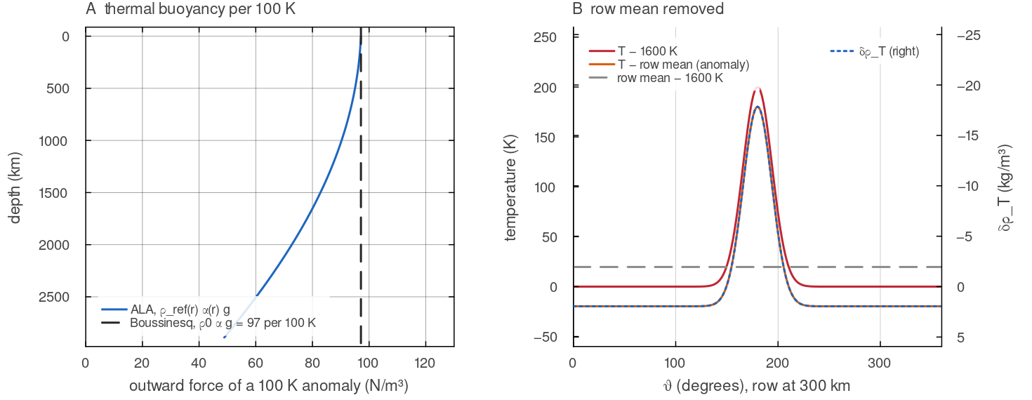
(A) Force per 100 K of lateral anomaly, ${\rho }_{\text{ref}}(r)\alpha (r)g$ from compressibility under ALA, falling from 97 N/m³ at the surface to 49 N/m³ at the base as the expansivity decreases, against the constant Boussinesq value ${\rho }_0\alpha g$. (B) One row at 300 km with a broad 200 K warm region. The row mean is 20 K above the background, so the anomaly peaks at 180 K and the rest of the row is 20 K cold; the dotted curve is the thermal density of compute_buoyancy on the right-hand axis, flipped so that it overlies the anomaly. Default shell, 64 × 256 cells. Script: docs/scripts/fig_buoyancy_sections.jl.

Phase transitions

The 410, 520 and 660 km analogues and post-perovskite enter as smooth phase functions ${\mathrm{\Gamma }}_k$ of pressure and temperature with their horizontal mean removed, $\delta {\rho }_{\text{phase}}+\delta {\rho }_{\text{Clap}}=\sum _k\mathrm{\Delta }{\rho }_k({\mathrm{\Gamma }}_k-⟨{\mathrm{\Gamma }}_k{⟩}_r)$, so they drive flow only through the temperature deflection of each boundary. cfg.useClaperonBuoyancy switches on the 410 and 660 analogues. cfg.usePhaseTransitionDensity adds the 520 km term (and post-perovskite with cfg.usePostPerovskite), plus the 410 and 660 terms when Clapeyron buoyancy is off; it acts only when cfg.useMeltingPhase is on, so a default run has no phase buoyancy. Each step has its own width, derived from the mesh at its own depth. Slopes, depths, density jumps, the mesh-derived width and the latent heat of the transitions are on the Phase changes page.

In words: ${\mathrm{\Gamma }}_k$ runs from 0 above transition $k$ to 1 below it, and $\mathrm{\Delta }{\rho }_k$ is the density jump across it. Subtracting the row mean $⟨{\mathrm{\Gamma }}_k{⟩}_r$ leaves a non-zero value only in cells whose phase differs from the average of their radius, which happens where temperature has moved the boundary. An exothermic transition (positive Clapeyron slope, the 410 and 520 km analogues) is crossed early by cold material and late by hot material, so it adds to the thermal buoyancy and helps flow through it. An endothermic one (negative slope, the 660 km analogue) does the reverse and opposes the thermal buoyancy, which is why the plume cell in the figure above ends up heavier than its row. The real transitions are only a few kilometres wide, much thinner than a convection cell, so the tanh width is a numerical choice tied to the mesh.

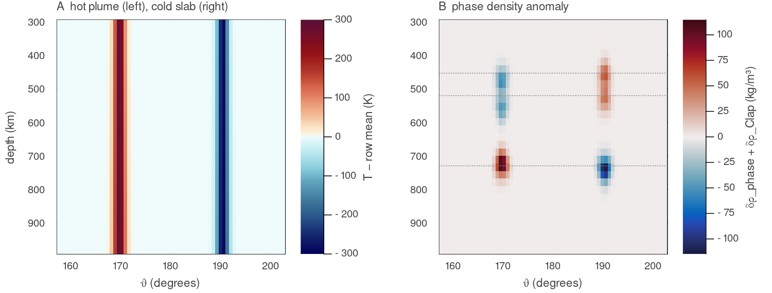
(A) Lateral temperature anomaly of a column 300 K hotter (left) and one 300 K colder (right) than the 1600 K adiabat below 200 km. (B) The phase part of compute_buoyancy (Clapeyron 410 and 660 terms plus the 520 term, phase field passed). The hot column is lighter at the exothermic 410 and 520 km analogues and denser at the endothermic 660 km analogue, and the cold column the reverse. Dotted lines mark the default depths 453, 520 and 730 km. Default shell, ALA pressure, 128 × 512 cells. Script: docs/scripts/fig_buoyancy_sections.jl.

Compositional buoyancy

Composition lives on the markers and is projected to cells as weighted cell means (basalt_evolution! when melting is on, project_marker_field_2d otherwise). Four fields enter $\delta {\rho }_C$:

$$\delta {\rho }_C=-\mathrm{\Delta }{\rho }_{\text{dep}}min(\frac{C_{\text{dep}}}{F_{\text{max}}},1)+\mathrm{\Delta }{\rho }_{\text{pile}}(C_{\text{pile}}-⟨C_{\text{pile}}{⟩}_r)+\mathrm{\Delta }{\rho }_{\text{ecl}}{C}_{\text{bas}}{f}_{\text{ecl}}(z,T)-\mathrm{\Delta }{\rho }_{\text{crust}}{X}_{\text{crust}}.$$

where

$$C_{\text{dep}}$$

is the depletion, the fraction of the parcel already extracted as melt, and $F_{\text{max}}$ = cfg.fertileFraction is the largest fraction that can be extracted, so $min(C_{\text{dep}}/F_{\text{max}},1)$ runs from 0 for fertile mantle to 1 for a fully depleted residue;

• $$C_{\text{pile}}$$

  is the fraction of thermochemical-pile material in the cell;

• $$C_{\text{bas}}$$

  is the basalt fraction and $f_{\text{ecl}}(z,T)$ the share of that basalt that has turned to eclogite at depth $z$;

• $$X_{\text{crust}}$$

  is the crust fraction defined below; and

• the four $\mathrm{\Delta }\rho$ are the density contrasts of the table, all positive, so the signs in the equation say which materials are light (residue, crust) and which are heavy (pile, eclogite).

Each term is linear in its composition field, so a cell half full of eclogite carries half the eclogite contrast. This represents each cell as a mixture of two end members whose densities differ by a fixed amount, and it lets the compositional fields be projected from the markers as simple cell means. The depletion term is capped at one, so a value of $C_{\text{dep}}$ above $F_{\text{max}}$ adds no further deficit.

term	parameter	default	meaning
depleted residue	cfg.depletionDensityAnomaly	50 kg m${}^{-3}$	deficit of the full residue, reached at $C_{\text{dep}}=F_{\text{max}}$ = cfg.fertileFraction (0.30)
thermochemical pile	mat.tcpile_drho	50 kg m${}^{-3}$	excess of pile material; lateral anomaly only
basalt / eclogite	cfg.basaltDensityAnomaly	200 kg m${}^{-3}$	excess of eclogite below the transition
crust	cfg.crustDensityAnomaly	0	deficit of crust relative to the mantle reference

Eclogite. $f_{\text{ecl}}(z,T)$ is the eclogite fraction of basalt. It is zero above cfg.eclogiteTransitionDepth (60 km), rising to one over the 20 km below it, with an optional temperature-gated metastability (cfg.useEclogiteKinetics). Its definition is on the Phase changes page.

Depleted residue. Melting leaves behind a residue that is poorer in iron and in the components that form garnet, and therefore lighter than the fertile mantle it came from. The default deficit of 50 kg m${}^{-3}$ for a fully depleted residue follows Jordan (1978) and Schutt & Lesher (2006). The term matters most where the residue is also cold. In a thick, depleted lithospheric root the compositional lightness works against the thermal heaviness, and the balance between the two decides whether the root is stable, sinks or spreads. Because the deficit is applied without removing a row mean, a row that is uniformly depleted feels only a change in pressure, and a depleted region drives flow only where it borders fertile mantle at the same depth.

Basalt and eclogite. Basalt produced by melting is lighter than the mantle while it stays at low pressure. Carried deeper, as part of a thickening crust, a delaminating lower crust or a cold drip, it transforms to eclogite and becomes one of the densest materials in the upper mantle (Irifune & Ringwood 1993). The transformation therefore turns a buoyant layer into a heavy one over a short depth interval, and is a common driver of lithospheric drips in models of planets without plate tectonics. MILEVA represents this with the depth ramp $f_{\text{ecl}}(z)$ and, optionally, with a temperature gate that keeps cold eclogite dense when it is carried back above the transition depth.

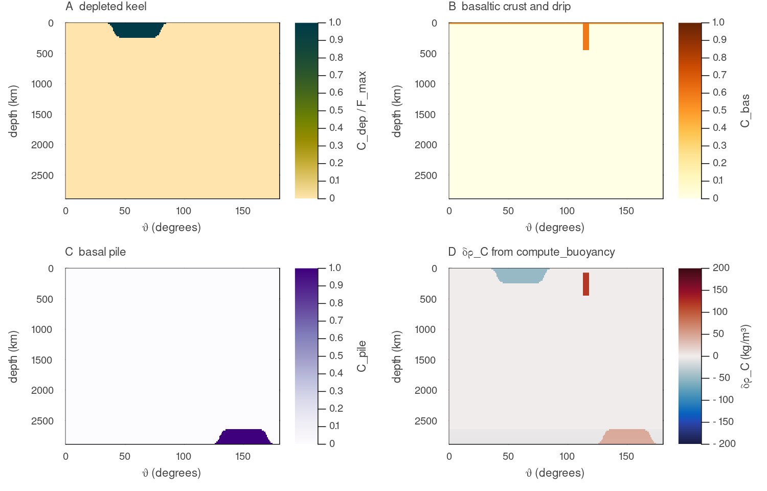
Half of the annulus with (A) a fully depleted keel 250 km thick, (B) a 30 km basaltic crust of fraction 0.5 and a drip of fraction 0.6 to 450 km depth, and (C) a 250 km high pile at the base. (D) The compositional density $\delta {\rho }_C$ of compute_buoyancy: the keel is 50 kg/m³ light, the crust is neutral (the default crust contrast is zero), the drip is 120 kg/m³ heavy below the eclogite ramp, and the pile is heavy inside and slightly light outside, because only its lateral anomaly enters. Default shell, 128 × 512 cells, uniform temperature. Script: docs/scripts/fig_buoyancy_sections.jl.

Crust as a material

The crust fraction (crust_fraction in physics/compute_buoyancy.jl) is the painted crust (the marker field C, projected as :continent) plus the basalt that sits above the eclogite transition, using the same 20 km ramp $f_{\text{ecl}}(z)$:

$$X_{\text{crust}}=\mathrm{clamp}(C_{\text{cont}}+C_{\text{bas}}[1-f_{\text{ecl}}(z)],0,1).$$

It lowers the density by cfg.crustDensityAnomaly (for example $3300-2800=500$ kg m${}^{-3}$) and, on the simple viscosity path, scales the viscosity by cfg.crustViscosityFactor (see Rheology). Both default to off.

Shallow basalt is neutral by default

With crustDensityAnomaly = 0 (the default) basalt shallower than the eclogite transition carries no density contrast; set this parameter to give the crust its buoyancy. The crust term exists in the 2-D buoyancy only; the 3-D dispatch has the depletion, pile and eclogite terms but no crust term.

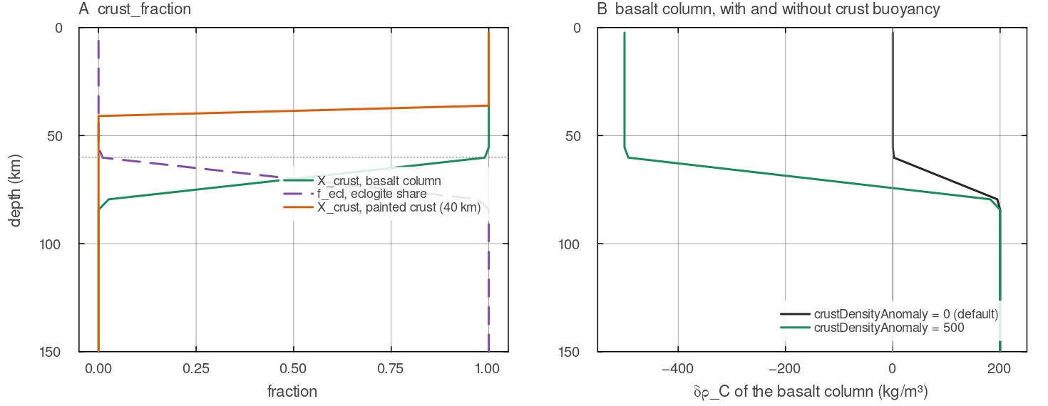
(A) crust_fraction for a column of basalt (fraction 1) and for 40 km of painted crust, with the eclogite share $f_{\text{ecl}}$ of the same 20 km ramp below cfg.eclogiteTransitionDepth (60 km, dotted). (B) $\delta {\rho }_C$ of the basaltic column from compute_buoyancy: with the default crustDensityAnomaly = 0 the basalt is neutral above 60 km, and with 500 kg/m³ it is 500 kg/m³ light there; below 80 km both carry the eclogite excess. 600 radial cells. Script: docs/scripts/fig_buoyancy_sections.jl.

Thermochemical piles

cfg.useThermochemicalPiles (default false) seeds dense basal material from cfg.tcPileInitTheta and tcPileHeightFrac and tracks it on markers (thermochemical_piles!, physics/thermochemical_piles.jl). Pile material is denser by mat.tcpile_drho, has its ductile viscosity scaled by mat.tcpile_eta_factor on the composite path, and carries cfg.radioHeatPileFactor times the mantle heat production. The fields cfg.tcPileDensityAnomaly and cfg.tcPileViscMult are not read by the buoyancy or the rheology; the live values are the mat.tcpile_* fields. If compute_buoyancy is called without a material table it uses the MaterialProperties defaults, so the pile excess is then the default mat.tcpile_drho.

Unlike the depletion and eclogite terms, the pile term is written as a lateral anomaly, $C_{\text{pile}}-⟨C_{\text{pile}}{⟩}_r$. Piles are a model for the large, compositionally distinct regions seismology finds at the base of Earth's mantle. Whether such material stays as a basal layer, gathers into piles or is entrained by plumes depends on its buoyancy number $B$ and on its viscosity relative to the mantle above it (Davaille 1999).

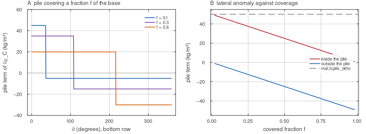
(A) The pile part of $\delta {\rho }_C$ along the bottom row for a pile covering 10, 30 and 60 per cent of the base. (B) Its value inside and outside the pile against the covered fraction $f$, which is $\mathrm{\Delta }{\rho }_{\text{pile}}(1-f)$ and $-\mathrm{\Delta }{\rho }_{\text{pile}}f$ because the row mean is removed. A pile that covered the whole base would drive no flow. From compute_buoyancy with the default mat.tcpile_drho = 50 kg/m³, 512 cells around. Script: docs/scripts/fig_buoyancy_sections.jl.

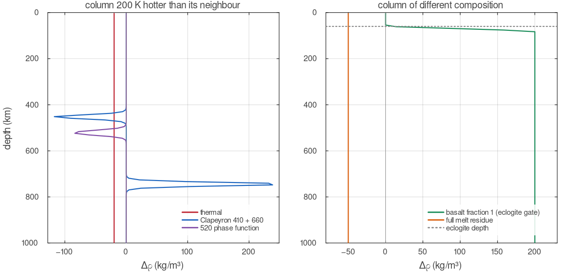
Each density term of compute_buoyancy, as the difference between a column carrying an anomaly and a reference column. Left: a column 200 K hotter, giving the thermal term and the deflection of the 410, 520 and 660 km phase functions (Clapeyron buoyancy on). Right: a fully basaltic column, neutral above the eclogite depth and 200 kg/m³ denser below it, and a fully depleted residue, 50 kg/m³ lighter at every depth.

Sticky air

cfg.useStickyAir overrides the top cfg.airThickness of cells with viscosity cfg.airViscosity and writes cfg.airDensity into the buoyancy field there (apply_sticky_air!, utils/sticky_air.jl). The value is written into an array of force densities, so with the default airDensity = 1.0 the air layer carries a buoyancy of 1 N m${}^{-3}$, effectively zero. See Free surface and isostasy.

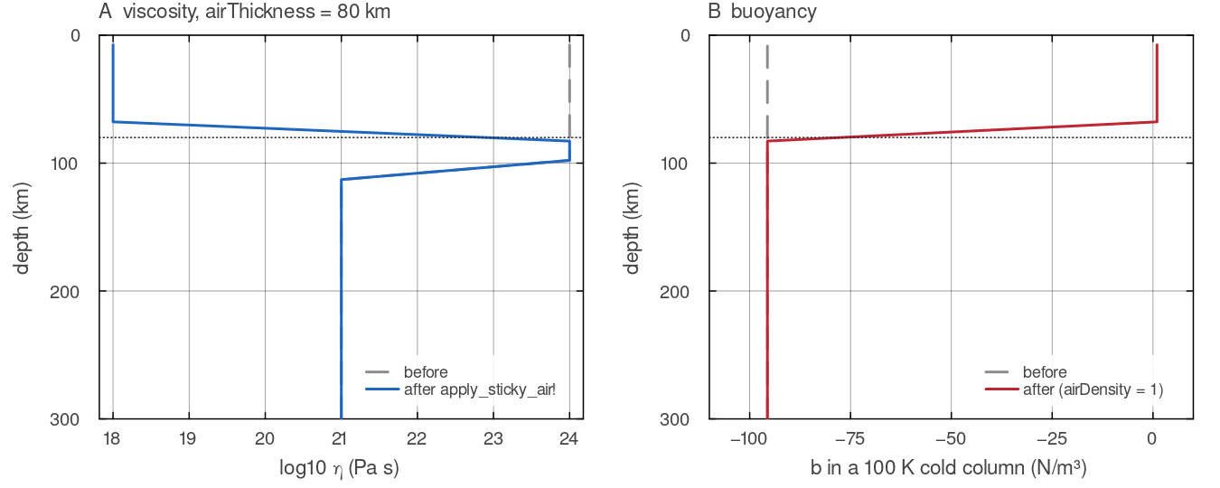
A column with a ${10}^{24}$ Pa s lid over ${10}^{21}$ Pa s mantle and a 100 K cold anomaly, before and after apply_sticky_air! with cfg.useStickyAir = true and the defaults airThickness = 80 km, airViscosity = ${10}^{18}$ Pa s, airDensity = 1. (A) Every cell whose centre lies in the top 80 km takes the air viscosity. (B) The same cells take a buoyancy of 1 N/m³ in place of the −95 N/m³ of the cold column. Default shell, 192 radial cells. Script: docs/scripts/fig_buoyancy_sections.jl.

Assumptions and simplifications

The buoyancy in MILEVA rests on the following choices. Each is standard in mantle-convection modelling and each can be relaxed only by changing the code.

• Uniform, radial gravity. $g$ = cfg.g is the same at every radius and points to the centre. In Earth's mantle gravity varies by about ten per cent between the surface and the core-mantle boundary (Dziewonski & Anderson 1981). The density anomalies do not modify the gravity field (no self-gravitation).

• Additive contributions. The total anomaly is the sum of thermal, phase and compositional parts. Cross effects, such as a thermal expansivity that depends on composition or a basalt density contrast that depends on temperature, are not included.

• Fixed compositional contrasts. Each compositional $\mathrm{\Delta }\rho$ is a constant. In reality the contrast of basaltic material changes with depth through its own sequence of phase changes, and below the 660 km transition it is briefly lighter than the surrounding mantle (Irifune & Ringwood 1993). MILEVA keeps the eclogite contrast constant below the transition ramp.

• Smooth phase transitions. Each phase change is a tanh step whose width is set by the mesh rather than by mineral physics, so that the force is resolved on the grid and continuous in temperature.

• Boussinesq or anelastic thermal term. The thermal term uses a constant ${\rho }_0\alpha$ under Boussinesq and the depth-dependent reference state under ALA and TALA; the phase and compositional terms are the same in all modes.

• Lateral means over a patch. In 3-D the row mean is taken over the $(\theta ,\varphi )$ cells of each Yin-Yang patch separately, not over the whole sphere.

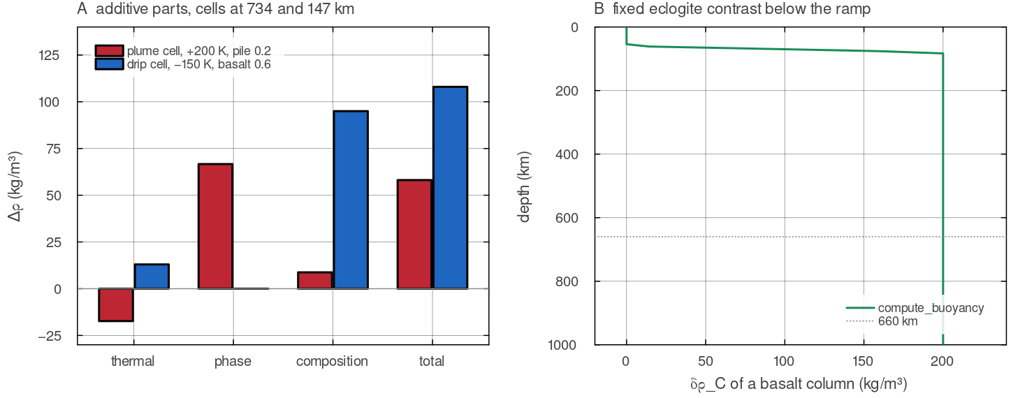
(A) The two example cells of the pipeline figure at the top of this page, split into the parts compute_buoyancy adds. The plume cell (734 km, +200 K, pile 0.2) sums −17.3, +66.7 and +8.8 to +58.1 kg/m³, and the drip cell (147 km, −150 K, basalt 0.6, depletion 0.15) sums +13.0 and +95.0 to +108.0 kg/m³. No term depends on another. (B) A basaltic column carries the same 200 kg/m³ eclogite excess at every depth below the 60 to 80 km ramp, including below 660 km, where real basaltic material changes its density again. Default shell. Script: docs/scripts/fig_buoyancy_sections.jl.

Diagnostics

Setting _BUOY_PARTS[] = true makes the next compute_buoyancy call keep its thermal, phase, Clapeyron and compositional parts in _BUOY_LAST[], so a peaked buoyancy field can be attributed to the term responsible. It is off by default and costs nothing when off.

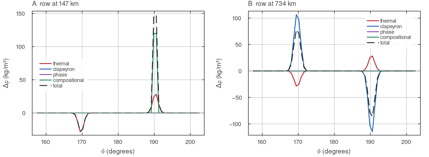
The parts stored in _BUOY_LAST[] after one call with _BUOY_PARTS[] = true, along a row at 147 km (A) and at 734 km (B), for a field with a hot plume (170°), a cold slab (190°) and a basaltic drip of fraction 0.6 inside the slab. At 147 km the drip's eclogite dominates; at 734 km the Clapeyron term of the 660 km analogue outweighs the thermal term and reverses the sign of the total in both columns. Default shell, ALA pressure, 128 × 512 cells. Script: docs/scripts/fig_buoyancy_sections.jl.

Where in the code

What	File, function
buoyancy, 2-D and 3-D	physics/compute_buoyancy.jl: compute_buoyancy, phase_transitions, _phase_density, _clap_width, crust_fraction
ALA thermal term	main_SphCon.jl, step 4
reference state	physics/compressibility.jl: compressibility
projection of depletion without melting	physics/basalt_evolution.jl: project_marker_field_2d
piles	physics/thermochemical_piles.jl: thermochemical_piles!
sticky air	utils/sticky_air.jl: apply_sticky_air!

Tests

• tests/test_crust_material.jl: the crust fraction, and that crustDensityAnomaly = 0 leaves the buoyancy unchanged.

• tests/test_depletion_projection.jl: a painted depletion reaches the grid when melting is off.

• tests/test_phase_transition_consistency.jl: the phase parameters are read from mat, a call without mat uses the MaterialProperties defaults, and each transition's width is taken at its own depth.

Key references

• Christensen, U. R. & Yuen, D. A. (1985). Layered convection induced by phase transitions. JGR 90, 10291-10300. doi:10.1029/JB090iB12p10291

• Tian, J., Tackley, P. J. & Lourenço, D. L. (2023). The tectonics and volcanism of Venus: new modes facilitated by realistic crustal rheology and intrusive magmatism. Icarus 399, 115539. doi:10.1016/j.icarus.2023.115539

• Jordan, T. H. (1978). Composition and development of the continental tectosphere. Nature 274, 544-548. doi:10.1038/274544a0

• Schutt, D. L. & Lesher, C. E. (2006). Effects of melt depletion on the density and seismic velocity of garnet and spinel lherzolite. JGR 111, B05401. doi:10.1029/2003JB002950

Further reading

• Schubert, G., Turcotte, D. L. & Olson, P. (2001). Mantle Convection in the Earth and Planets. Cambridge University Press. doi:10.1017/CBO9780511612879. The standard reference for the physics of mantle convection, including the Boussinesq approximation, thermal expansivity and compositional layering.

• Turcotte, D. L. & Schubert, G. (2014). Geodynamics, 3rd edn. Cambridge University Press. doi:10.1017/CBO9780511843877. Stokes flow, the Stokes velocity of a sphere, and the buoyancy of thermal and compositional anomalies at an introductory level.

• Jarvis, G. T. & McKenzie, D. P. (1980). Convection in a compressible fluid with infinite Prandtl number. J. Fluid Mech. 96, 515-583. doi:10.1017/S002211208000225X. The anelastic approximation behind the ALA thermal term.

• Dziewonski, A. M. & Anderson, D. L. (1981). Preliminary reference Earth model. Phys. Earth Planet. Inter. 25, 297-356. doi:10.1016/0031-9201(81)90046-7. Radial density, gravity and the density steps of the transition zone.

• Irifune, T. & Ringwood, A. E. (1993). Phase transformations in subducted oceanic crust and buoyancy relationships at depths of 600-800 km in the mantle. Earth Planet. Sci. Lett. 117, 101-110. doi:10.1016/0012-821X(93)90120-X. The density of basaltic material relative to the mantle with depth.

• Davaille, A. (1999). Simultaneous generation of hotspots and superswells by convection in a heterogeneous planetary mantle. Nature 402, 756-760. doi:10.1038/45461. Laboratory experiments on the stability of dense layers as a function of the buoyancy number.

• NASA Venus Fact Sheet (D. R. Williams, NSSDCA), https://nssdc.gsfc.nasa.gov/planetary/factsheet/venusfact.html. Bulk parameters of Venus, including surface gravity 8.87 m s${}^{-2}$.