Plume planforms in a 3-D shell

Basally heated, isoviscous convection in a full spherical shell on the Yin-Yang grid. The Rayleigh number sets how many plumes the shell holds and how thin they are. At Ra = 10⁴ a few broad upwellings, at 10⁵ more of them, at 10⁶ many thin plumes rising from a thin hot boundary layer, separated by a network of cold sheets.

The driver is examples/yinyang_convection_3d.jl. It runs on exactly two MPI ranks and is meant for a cluster; the HPC page has the batch scripts.

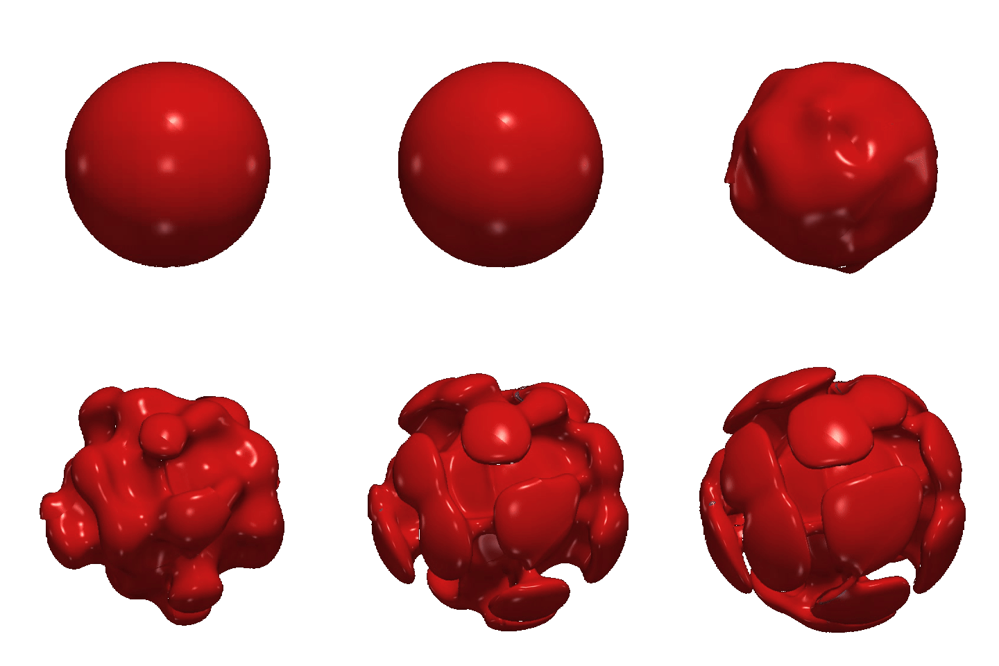
A MILEVA run at Ra = 10⁶: the hot-temperature isosurface shows plumes rising from the core-mantle boundary and spreading beneath the surface.

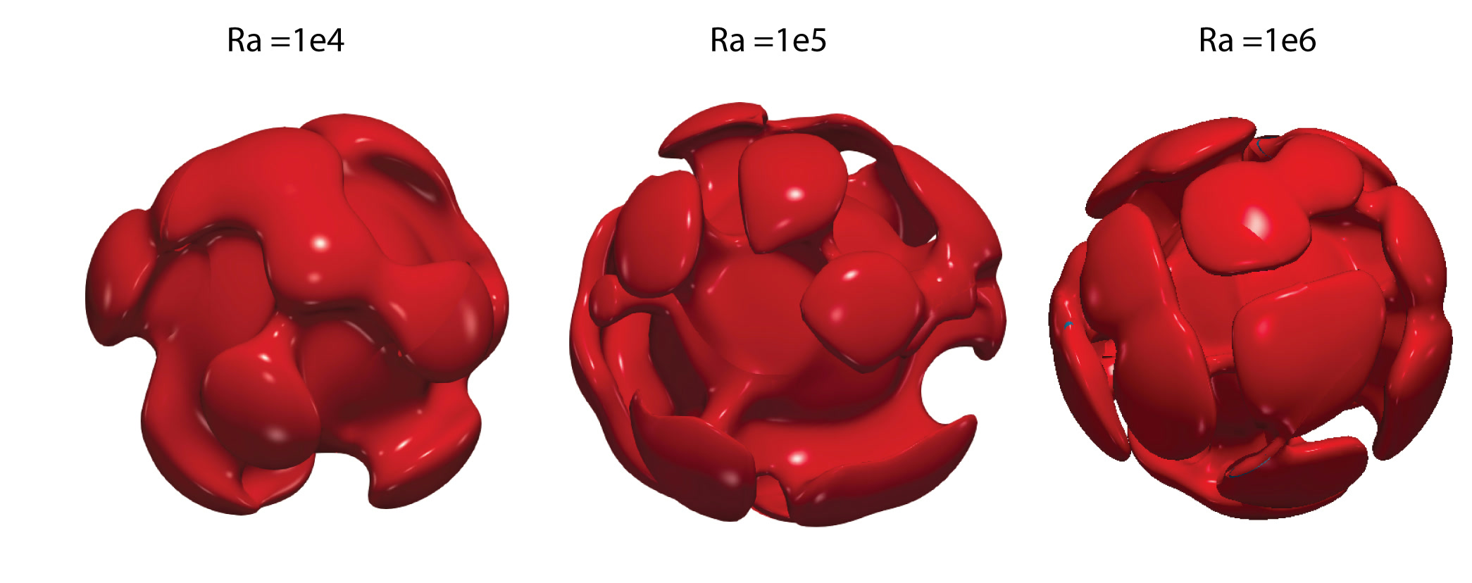
MILEVA 3-D Yin-Yang spherical shell, hot-temperature isosurfaces at Ra = 10⁴, 10⁵, 10⁶. Plumes become more numerous and narrower as Ra grows.

The model

$$\mathrm{\nabla }\cdot \left(2\eta \dot{\mathit{\epsilon }}\right)-\mathrm{\nabla }p={\rho }_0\alpha (T-T_{\mathrm{mid}})g\hat{\mathbf{r}},\mathrm{\nabla }\cdot \mathbf{v}=0,\frac{\partial T}{\partial t}+\mathrm{\nabla }\cdot (\mathbf{v}T)-T\mathrm{\nabla }\cdot \mathbf{v}=\kappa {\mathrm{\nabla }}^{2}T,$$

in a shell with $R_{\mathrm{in}}=1220$ km, $R_{\mathrm{out}}=2220$ km, i.e. the Hernlund & Tackley (2008) aspect ratio $f=0.5495$ and a 1000 km layer, for which their Table 1 lists values for the 3-D spherical shell:

Ra	$\eta$ [Pa s]	Nu (H&T 3-D shell)	$V_{\mathrm{rms}}$ (H&T 3-D shell)
${10}^4$	$9.7\times {10}^{22}$	3.85	42.3
${10}^5$	$9.7\times {10}^{21}$	7.27	160
${10}^6$	$9.7\times {10}^{20}$	15.9	625

These are the reference values for a time-averaged comparison.

Grid and solver

item	value	where
grid per patch	Nr × Nth × 3 Nth: 64 × 32 × 96 (Ra 10⁴), 64 × 48 × 144 (10⁵), 96 × 72 × 216 (10⁶)	MILEVA_NR, MILEVA_NTH
radial spacing	refined toward both walls, cfg.amrStretchFactor = 2	utils/setup_grid.jl
Yin-Yang overlap	basic overlap, no θ-buffer (cfg.δ_yy = 0), cfg.useMinOverlapGrid = false	Yin-Yang grid
MPI layout	Phase A: rank 0 = Yin, rank 1 = Yang	parallel/mpi_init.jl
Stokes	solve_stokes_distributed!(...; mode = :phase_a), i.e. multigrid_stokes_mpi!	solvers/solve_stokes_distributed.jl, solvers/multigrid_stokes_mpi.jl
inner solver	FGMRES (tol ${10}^{-6}$, ≤ 300 iterations) (restart 50) with a geometric V-cycle, two pre- and two post-SCGS sweeps (multigrid_stokes_mpi.jl, not the 5/5 of the serial path), Galerkin coarse operators, mgLevels = 4	Multigrid
patch coupling	8 Jacobi-Schwarz rounds per solve with damped Anderson acceleration (MILEVA_NSCHWARZ)	multigrid_stokes_mpi!
advection	second-order TVD (van Leer) on the grid, advect_temperature_3d_tvd!	utils/advect_temperature.jl
diffusion	backward Euler, wall temperatures held at the faces through a half-cell ghost	diffuse_temperature(...; implicit = true)
temperature seam	θ-wall cells overwritten with the peer's interpolated temperature after every step	yy_sync_T_walls_mpi! in parallel/yinyang_mpi.jl
time step	advective CFL in all three directions, safety 0.4; dtMax = ${10}^{-4}{D}^2/\kappa$ for the conductive start	compute_timestep plus a longitude term in the driver

Why exactly two ranks. Among the modes of solve_stokes_distributed!, Phase A is the only one that solves Stokes with multigrid; the multi-rank-per-patch modes are MUMPS-direct (:direct, :b4p) or block-Jacobi Krylov (:iter, :rich). MILEVA's rule is that 3-D Stokes is always multigrid, so the driver refuses any other rank count and the job scales through Julia threads within each rank, which the SCGS smoother uses.

Initial condition. The spherical conductive profile plus a perturbation

$$T(r,\mathbf{n})=T_{\mathrm{surf}}+\mathrm{\Delta }T\frac{1/r-1/R_{\mathrm{out}}}{1/R_{\mathrm{in}}-1/R_{\mathrm{out}}}+A\sin (\pi \xi )\frac{\sum _{w=1}^{48}\sin ({\mathbf{k}}_w\cdot \mathbf{n}+{\varphi }_w)}{\sqrt{24}},\xi =\frac{r-R_{\mathrm{in}}}{D},$$

where $\mathbf{n}$ is the unit position vector in physical Cartesian coordinates, the 48 wavevectors ${\mathbf{k}}_w$ have random directions and lengths between 2 and 12, and $A$ = 20 K (MILEVA_SEED_AMP). Because the pattern is a function of physical position drawn from one seed, Yin and Yang start from the same field in their overlap, and because it has no preferred wavenumber the planform selects itself. The $\sin (\pi \xi )$ factor vanishes at both walls, so the wall heat flux starts at its conductive value: the smoke runs below start at $\mathrm{Nu}=1.00$.

Diagnostics

Every MILEVA_LOGEVERY steps the driver appends to diagnostics_3d.csv:

column	definition
t_diff	time in units of $D^2/\kappa$
Vrms_nd	$\sqrt{\int |\mathbf{v}{|}^{2}dV/\int dV}D/\kappa$, cell-centred velocities, $dV=r^2\sin \theta drd\theta d\varphi$
Nu_top, Nu_bot	area-weighted mean wall gradient $(T_{\mathrm{bc}}-T_{\mathrm{wall}\mathrm{cell}})/(\text{half cell})$ over the spherical conductive gradient $\mathrm{\Delta }T/[r^2(1/R_{\mathrm{in}}-1/R_{\mathrm{out}})]$ at the same wall
Tmean_nd	volume-mean $(T-T_{\mathrm{surf}})/\mathrm{\Delta }T$
fgmres_iters, final_res	inner FGMRES iterations and relative residual of the last Schwarz round
schwarz_res	smallest relative velocity change between Schwarz rounds; the solver returns that iterate
divMax	the solver's own nondimensional divergence diagnostic (unpack_stokes_3d)

The sums run over both patches with one MPI.Allreduce. Yin and Yang overlap by about 6 % of the sphere and that overlap is counted twice, so these are patch-weighted means rather than exact sphere integrals.

Running it

The Rayleigh number and everything else are environment variables (the full list is in the driver header). Locally, with the mpiexec that MPI.jl ships:

MILEVA_RA=1e5 JULIA_NUM_THREADS=4 \
  julia --project=. -e 'using MPI; run(`$(mpiexec()) -n 2 $(Base.julia_cmd()) --project=. examples/yinyang_convection_3d.jl`)'

On a cluster, the array script runs the three Rayleigh numbers and chains segments across the queue's time limit:

julia --project=. hpc/plan_3d.jl 32           # memory per rank for each case
hpc/submit_3d_chain.sh 4                       # 4 chained 48 h segments of the array

A segment stops cleanly before its time limit (MILEVA_WALLTIME_H), writing a checkpoint per rank; the next resumes with MILEVA_RESUME=latest. A case that reaches its end (MILEVA_TMAX diffusion times, default 0.2, or MILEVA_MAXSTEPS) writes FINISHED in its output directory and later segments skip it. Open the .pvd in ParaView; each step is a .vtm holding the Yin and Yang .vts blocks, with fields T, eta, V and mpi_patch.

Cost

Measured on a laptop with 2 threads per rank:

grid per patch	DOFs per patch	Stokes per step	FGMRES its per solve	Schwarz residual
8 × 8 × 24 (smoke)	6 528	1.2 to 2.0 s	34 to 35	$2\times {10}^{-3}$ to $3\times {10}^{-3}$ (Ra 10⁴)
16 × 16 × 48 (smoke), 8 rounds	50 688	11 to 13 s	36 to 37	$9\times {10}^{-3}$
16 × 16 × 48 (smoke), 4 rounds	50 688	6 s	36 to 37	$5\times {10}^{-2}$

The first step of every run also pays about 20 s of compilation. Halving the Schwarz rounds halves the cost and leaves the seam five times less converged; in those four steps $V_{\mathrm{rms}}$ differed by under 1 %. The cost per Schwarz round is roughly linear in the DOF count, which puts the default grids at minutes per step on two threads per rank. The Ra = 10⁵ default grid has 1.8 million DOFs per patch and needs about 1.8 GB per rank. A short probe on the cluster gives the time per step:

MILEVA_MAXSTEPS=5 MILEVA_LOGEVERY=1 sbatch --array=1 --time=02:00:00 hpc/yinyang_convection_3d.slurm

and scale the seconds per step it reports by the step count the CFL condition implies.

Notes

• Temperature lives on the grid and is advected by TVD; there is no marker field in this example.

• Both patches are written in full, so in ParaView the overlap shows two values at one place, and the diagnostics count the overlap twice, as described above. Next to a patch's φ-walls, read temperatures from the peer patch, which holds them in its interior. See Yin-Yang grid for how the patches are coupled.

Smoke test

A quick check on 2 ranks × 2 threads:

MILEVA_NR=8 MILEVA_NTH=8 MILEVA_MGLEVELS=2 MILEVA_MAXSTEPS=3 MILEVA_LOGEVERY=1 \
  julia --project=. -e 'using MPI; run(`$(mpiexec()) -n 2 $(Base.julia_cmd()) --project=. examples/yinyang_convection_3d.jl`)'

3 steps at Ra = 10⁵ in 37 s of wall time. FGMRES converged every inner solve (34 to 35 iterations to a relative residual below ${10}^{-6}$); temperature and velocity were finite on both patches; Nu started at 1.00 and $V_{\mathrm{rms}}$ grew from 43 to 59 over the three steps as the perturbation began to grow. A resume from the step-3 checkpoint continued the PVD collection, a wall-time stop wrote a checkpoint and no FINISHED, and the dry run of hpc/yinyang_convection_3d.slurm through mpiexecjl ran and finished.