Benchmarks and verification

MILEVA's 2-D science path is the spherical annulus (radial measure $r^{2}dr$, Hernlund & Tackley 2008) and its 3-D path is the Yin-Yang spherical shell. Evidence that the code solves the equations it claims to solve comes in three kinds, and this page keeps them apart:

Kind	What it shows	Examples
Verification against published results	The same physical problem, solved by an independent code in the same geometry, gives the same numbers as the published tables.	Hernlund & Tackley (2008) spherical-annulus tables; the Annulus column of Fleury et al. (2024); the Kageyama & Sato (2004) Yin-Yang rotation formulas.
Verification against exact identities	A property every correct discretisation must satisfy, independent of any reference value: conservation, an exact null mode, an energy identity.	Nu = 1 on conduction, closed energy budget, work = dissipation, rigid rotation annihilated, $G=-B^{\mathsf{T}}$.
Regression	The code agrees with itself: two solvers on the same matrix, the serial and distributed assemblies, a stored earlier result. It protects against change, not against a wrong operator.	MUMPS against UMFPACK, multigrid against MUMPS, serial against distributed 3-D assembly.

Same geometry

The 2-D path is compared only with spherical-annulus references (Hernlund & Tackley 2008; the Annulus column of Fleury et al. 2024). Cartesian box benchmarks, cylindrical annulus cases and Fleury et al.'s scaled cylinder column describe other geometries and are not used as targets.

Summary

Every spherical-annulus case with a published reference, at the finest grid run, against the reference value. Nu is ${\mathrm{Nu}}_{\mathrm{t}\mathrm{o}\mathrm{p}}$, $V_{\mathrm{r}\mathrm{m}\mathrm{s}}$ is in units of $\kappa /D$ and $⟨T⟩$ is the nondimensional volume mean over the $r^2$ measure, all time averaged; Δ is MILEVA relative to the reference. Details, resolution series and notes for each row are in the sections below.

Case	Reference	Grid	Nu	Nu ref.	ΔNu	$V_{\mathrm{r}\mathrm{m}\mathrm{s}}$	$V_{\mathrm{r}\mathrm{m}\mathrm{s}}$ ref.	Δ$V_{\mathrm{r}\mathrm{m}\mathrm{s}}$	$⟨T⟩$	$⟨T⟩$ ref.	Δ$⟨T⟩$
Basal heating, Ra ${10}^4$, isoviscous	H&T 2008, Table 1	128 × 1024	4.05	4.18	−3.1 %	35.0	37.7	−7.2 %
Basal heating, Ra ${10}^5$, isoviscous	H&T 2008, Table 1	64 × 512	7.70	7.39	+4.2 %	161.8	160	+1.1 %
Basal heating, Ra ${10}^5$, contrast ${10}^6$	H&T 2008, Table 2	64 × 512	5.18	5.71	−9.3 %	535.8	463	+15.7 %
Internal heating, Ra ${10}^4$	H&T 2008, Table 3	64 × 512				23.6	23.5	+0.4 %	0.310	0.308	+0.6 %
Internal heating, Ra ${10}^5$	H&T 2008, Table 3	64 × 512				75.8	78.5	−3.4 %	0.351	0.349	+0.6 %
Internal heating, Ra ${10}^6$	H&T 2008, Table 3	64 × 512				251.5	265	−5.1 %	0.341	0.350	−2.6 %
Basal heating, Ra ${10}^4$, $f=0.6$	Fleury et al. 2024, Annulus	64 × 512	4.39	4.63	−5.2 %	39.5	46.6	−15.2 %	0.295	0.283	+4.2 %
Basal heating, Ra ${10}^5$, $f=0.6$	Fleury et al. 2024, Annulus	64 × 512	9.36	8.99	+4.1 %	176.7	189.2	−6.6 %

Blank cells: an internally heated shell with an insulating core has no basal Nu, and the mean temperature has not yet been extracted from the basally heated runs. The two $f=0.4$ runs of Fleury et al. are left out because they have not converged. The references give their time-dependent cases as means with a peak-to-peak spread (H&T's $V_{\mathrm{r}\mathrm{m}\mathrm{s}}$ spread is ±90 at contrast ${10}^6$, 36 and 160 for internal heating at Ra ${10}^5$ and ${10}^6$), and the seeded planform moves Nu at Ra ${10}^5$ by up to 8 %, so differences of that size are within what the references themselves resolve. The internally heated rows at Ra ${10}^4$ and ${10}^5$ and the basally heated row at Ra ${10}^5$ are from runs that settled in the planform of Hernlund & Tackley's Fig. 3; in the other planforms the same cases differ by up to 20 %, as discussed below.

Running the benchmark driver

benchmarks/hernlund_tackley_annulus.jl sets up the reference problem from scratch: it clears every optional physics flag, then switches on only what the case needs.

# case, Nr, seeded wavenumber m (default 6); Nt = 8 Nr
julia --project=. benchmarks/hernlund_tackley_annulus.jl HT4 64
julia --project=. benchmarks/hernlund_tackley_annulus.jl HT5 128 6
julia --project=. benchmarks/hernlund_tackley_annulus.jl HTV5 64

# Fleury et al. (2024) annulus, Ra = 10^k, aspect ratio from MILEVA_F
MILEVA_F=0.6 julia --project=. benchmarks/hernlund_tackley_annulus.jl FL5 64

Case	Ra	Viscosity	Reference
HT4, HT5, HT6	${10}^4$, ${10}^5$, ${10}^6$	isoviscous	H&T 2008 Table 1
HTV5, HTV6	${10}^5$, ${10}^6$	$\eta =\exp [13.8156(0.5-T^{\prime })]$, contrast ${10}^6$	H&T 2008 Table 2
FL4 … FL8	${10}^4$ … ${10}^8$	isoviscous	Fleury et al. 2024, benchmarks/reference/fleury2024/

The setup is a Boussinesq, basally heated shell with free-slip walls, isothermal boundaries, no net rotation and a uniform grid. The layer is 1000 km thick with $f=r_{\mathrm{i}\mathrm{n}}/r_{\mathrm{o}\mathrm{u}\mathrm{t}}=1.22/2.22=0.5495$ for the H&T cases, and the viscosity is chosen to give the requested

$$\mathrm{Ra}=\frac{{\rho }_{0}g\alpha \mathrm{\Delta }T{D}^3}{\kappa \eta }.$$

The variable-viscosity cases use the Frank-Kamenetskii "simple" form with ${\theta }_{FK}=\ln {10}^6$ and $\eta ={\eta }_{\mathrm{R}\mathrm{a}}$ at $T^{\prime }=0.5$. The run goes to 0.6 thermal diffusion times ($D^2/\kappa$ is 31 688 Myr here), averages ${\mathrm{Nu}}_{\mathrm{t}\mathrm{o}\mathrm{p}}$ and $V_{\mathrm{r}\mathrm{m}\mathrm{s}}$ (in units of $\kappa /D$) over the last third, and fits a straight line through that window. If the trend exceeds the larger of 2 % (Nu) / 5 % ($V_{\mathrm{r}\mathrm{m}\mathrm{s}}$) and the reference's own published fluctuation, it prints a NOT CONVERGED flag. Output goes to output/benchmarks/ht2008_<case>_N<Nr>…/, including diagnostics.csv with the energy budget.

These runs take hours to days at Nr = 64 and above. Use MILEVA_MAXSTEPS=<n> and MILEVA_OUTTAG=<tag> for short probes.

The "T on grid (TVD)" row below is reproduced with the env knob MILEVA_TGRID=1, which sets cfg.temperatureOnGrid = true (TVD advection on the grid) and adds the suffix _gridT to the output directory:

MILEVA_TGRID=1 julia --project=. benchmarks/hernlund_tackley_annulus.jl HT5 64

Hernlund & Tackley (2008), spherical annulus

Reference values (Hernlund & Tackley 2008, 32 × 256). The 3-D column is the same study's spherical shell, shown for comparison with the annulus geometry.

Case	Nu annulus	$V_{\mathrm{r}\mathrm{m}\mathrm{s}}$ annulus	Nu 3-D shell	$V_{\mathrm{r}\mathrm{m}\mathrm{s}}$ 3-D shell
Ra ${10}^4$, isoviscous	4.18	37.7	3.85	42.3
Ra ${10}^5$, isoviscous	7.39	160	7.27	160
Ra ${10}^6$, isoviscous	14.4	640	15.9	625
Ra ${10}^5$, contrast ${10}^6$	5.71 ± 0.1	463 ± 90	6.30	405
Ra ${10}^6$, contrast ${10}^6$	10.1 ± 0.1	1390 ± 780	9.7	1804

The ± values are the paper's peak-to-peak spread for the time-dependent cases.

Measured

Seeded wavenumber $m=6$ unless stated. Nu is the time-averaged ${\mathrm{Nu}}_{\mathrm{t}\mathrm{o}\mathrm{p}}$; budget_resid is the energy-budget residual from diagnostics.csv (see below). Nr = 32 is the reference's own resolution and is listed as the low end of the resolution series.

Case	Nr × Nt	Nu MILEVA	Nu H&T	$V_{\mathrm{r}\mathrm{m}\mathrm{s}}$ MILEVA	$V_{\mathrm{r}\mathrm{m}\mathrm{s}}$ H&T	Notes
Ra ${10}^4$	32 × 256	4.24	4.18	35.4	37.7	steady, converged
Ra ${10}^4$	64 × 512	4.14	4.18	35.1	37.7	steady, converged
Ra ${10}^4$	128 × 1024	4.05	4.18	35.0	37.7	Nu_top/Nu_bot 4.052/4.011, budget_resid −0.0004
Ra ${10}^5$	32 × 256	8.76	7.39	156.9	160	time dependent, budget_resid 0.0000
Ra ${10}^5$	64 × 512	8.88	7.39	158.2	160	converged flag
Ra ${10}^5$	128 × 1024	8.90	7.39	159.6	160	time dependent, Nu_top/Nu_bot 8.97/8.96, budget_resid −0.001
Ra ${10}^5$, T on grid (TVD)	64 × 512	8.97	7.39	161.2	160	temperatureOnGrid = true, budget_resid +0.0108
Ra ${10}^5$, $m=4$	64 × 512	9.05	7.39	176.2	160	Nu_top/Nu_bot 9.05/9.09
Ra ${10}^5$, $m=8$	64 × 512	8.40	7.39	156.4	160	time dependent, budget_resid −0.0010
Ra ${10}^5$, $m=3$	64 × 512	7.70	7.39	161.8	160	three plumes and three downwellings from 15 Gyr, as in H&T Fig. 3; Nu_top/Nu_bot 7.68/7.70 over that state, budget_resid −0.0005
Ra ${10}^5$, contrast ${10}^6$	32 × 256	4.66	5.71 ± 0.1	440.6	463 ± 90	time dependent
Ra ${10}^5$, contrast ${10}^6$	64 × 512	5.18	5.71 ± 0.1	535.8	463 ± 90	time dependent, Nu_top/Nu_bot 5.183/5.161, budget_resid +0.0015

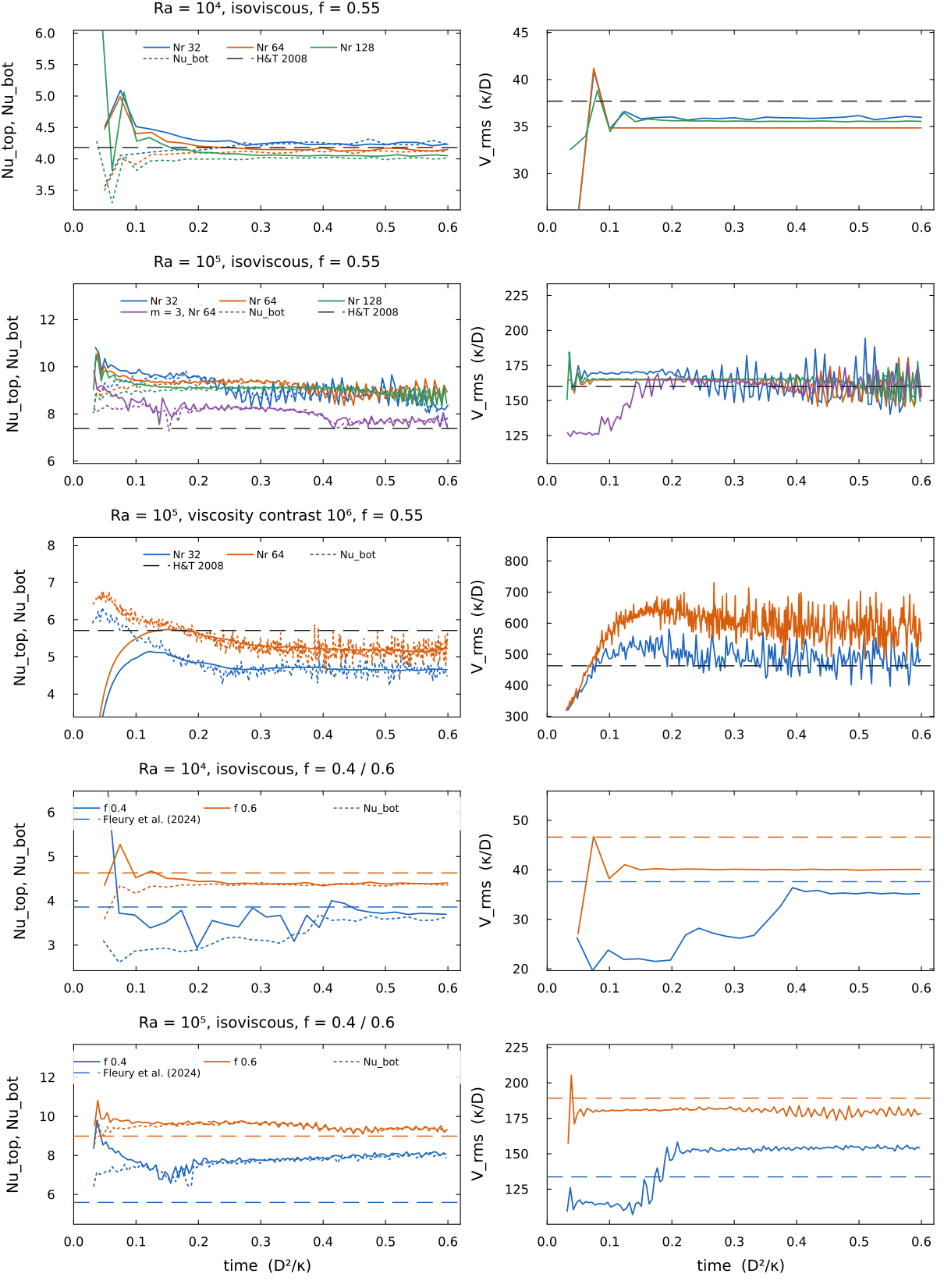
Time series from each run's diagnostics.csv over 0.6 thermal diffusion times, seeded $m=6$ except the $m=3$ run in the Ra ${10}^5$ row, whose Nu falls step by step as its plumes merge into the three of the reference run: ${\mathrm{Nu}}_{\mathrm{t}\mathrm{o}\mathrm{p}}$ solid, ${\mathrm{Nu}}_{\mathrm{b}\mathrm{o}\mathrm{t}}$ dotted, $V_{\mathrm{r}\mathrm{m}\mathrm{s}}$ in units of $\kappa /D$, published reference values dashed. The Nr = 64 runs of the first two rows are read from the run log, which prints $V_{\mathrm{r}\mathrm{m}\mathrm{s}}$ to two decimals in cm/yr, hence the steps in those curves. The bottom two rows are the Fleury et al. (2024) cases of the next section, with each aspect ratio's Fleury et al. (2024) value in the matching colour.

How to read it:

• Ra = ${10}^4$. Nu converges from above through the reference value (4.24, 4.14, 4.05 at Nr = 32, 64, 128, reference 4.18). The reference itself was computed at 32 × 256. $V_{\mathrm{r}\mathrm{m}\mathrm{s}}$ is 35.4, 35.1, 35.0 against 37.7, steady with resolution.

• Ra = ${10}^5$. Nu depends on the planform, not on the resolution. Runs seeded with $m=6$ keep many narrow cells and give Nu 8.76, 8.88, 8.90 from Nr = 32 to 128 (the grid TVD path gives the same, 8.97), 20 % above the reference. Hernlund & Tackley's Fig. 3 shows three plumes and three downwellings for this case. A run seeded with $m=3$ starts with about ten plumes, which merge over 15 Gyr into exactly that pattern, and Nu falls with each merger, from 9.2 to 7.70 (+4.2 %), with $V_{\mathrm{r}\mathrm{m}\mathrm{s}}$ 161.8 (+1.1 %). Wider cells carry heat less efficiently, so the cell count sets Nu. Fleury et al. (2024, their Table S3) obtain 7.16 and 160.0 for this case with GAIA. The seeded $m=4$ and $m=8$ runs (9.05 and 8.40) were averaged without checking which planform they had reached.

• Ra = ${10}^5$ at contrast ${10}^6$ (the case that exercises the variable-viscosity operator): $V_{\mathrm{r}\mathrm{m}\mathrm{s}}$ at Nr = 64 is 535.8 against the paper's 463 ± 90, and Nu rises toward the reference with resolution (4.66 at Nr = 32, 5.18 at Nr = 64, reference 5.71 ± 0.1).

• Ra = ${10}^6$ (HT6, HTV6): the driver supports these cases; no measurement is listed yet.

Internal heating (Table 3)

Purely internally heated, isoviscous, insulating core, the same shell, run with examples/annulus_internal_heating_2d.jl at 64 × 512, seeded $m=3$ at Ra ${10}^4$ and ${10}^5$ and $m=6$ at Ra ${10}^6$, averaged over the last third of 0.3 diffusion times (Internally heated convection). $⟨T{⟩}^{\prime }$ is the volume mean over the $r^2$ measure, $(⟨T⟩-T_{\mathrm{s}})/\mathrm{\Delta }T$.

Ra	$H^{\prime }$	$⟨T{⟩}^{\prime }$ MILEVA	$⟨T{⟩}^{\prime }$ H&T	$V_{\mathrm{r}\mathrm{m}\mathrm{s}}$ MILEVA	$V_{\mathrm{r}\mathrm{m}\mathrm{s}}$ H&T	Notes
${10}^4$	3.4	0.310	0.308	23.6	23.5	seeded $m=3$; three downwellings, steady from 3 Gyr
${10}^4$	3.4	0.278	0.308	19.8	23.5	seeded $m=6$; six downwellings, steady
${10}^5$	6.6	0.351	0.349	75.8	78.5 (peak to peak 36)	seeded $m=3$; five to six downwellings, reorganises near 8 Gyr, budget_resid +0.0004
${10}^5$	6.6	0.351	0.349	69.4	78.5 (peak to peak 36)	seeded $m=6$; budget_resid −0.0006
${10}^6$	14.0	0.341	0.350	251.5	265 (peak to peak 160)	time dependent (190 to 360), budget_resid 0.0000

In every case the surface heat flow equals the heat produced to within 0.4 %.

When quoting these numbers, state the seeded wavenumber cfg.m_wavenumber: more than one planform is stable at these Rayleigh numbers and the seed decides which one the run lands in. At Ra ${10}^4$ this is the whole difference: the $m=6$ run holds six cells and is 16 % slow and 10 % cold, while the $m=3$ run lands in the three downwellings of Hernlund & Tackley's Fig. 3 and agrees to within 1 % in both. At Ra ${10}^5$ the seed does not persist; both runs end in five to six cells, as in the reference figure, and differ only in $V_{\mathrm{r}\mathrm{m}\mathrm{s}}$. The reference has no error bars or convergence study, so the comparison is verification against published results.

Fleury et al. (2024), Annulus column

Fleury, Plesa, Hüttig & Breuer (2024, G3 25, doi 10.1029/2023GC011114) solved basally heated isoviscous convection in the 3-D sphere, the spherical annulus and a scaled cylinder, for $f=0.2$ to 0.8 and Ra = ${10}^4$ to ${10}^8$. Their tables (Zenodo doi 10.5281/zenodo.8047757) are in benchmarks/reference/fleury2024/, copied unmodified; the driver reads only the Annulus column. Their definitions match H&T (measure $2r^{2}drd\varphi$, same Ra, ${\mathrm{Nu}}_{\mathrm{t}\mathrm{o}\mathrm{p}}$ normalised by $f$). Two differences matter when comparing: Fleury et al. start from a 5 % random perturbation with an unreported planform (MILEVA seeds $m=6$), and their top gradient is a one-sided difference between the last two shells.

Measured at Nr × Nt = 64 × 512:

Case	$f$	MILEVA Nu (top/bot)	Fleury et al. Nu	MILEVA $V_{\mathrm{r}\mathrm{m}\mathrm{s}}$	Fleury et al. $V_{\mathrm{r}\mathrm{m}\mathrm{s}}$	$⟨T⟩$ MILEVA / Fleury et al.	Notes
Ra ${10}^4$	0.4	3.76 (3.74/3.60)	3.86	34.0	37.6	0.184 / 0.167	not converged (Nu_top and Nu_bot still apart)
Ra ${10}^4$	0.6	4.39 (4.39/4.37)	4.63	39.5	46.6	0.295 / 0.283
Ra ${10}^5$	0.6	9.36 (9.36/9.33)	8.99	176.7	189.2	n/a	converged, budget_resid −0.001
Ra ${10}^5$	0.4	8.03 (7.98/7.91)	5.59	148.2	133.7	n/a	not converged (Nu still trending)

The $f=0.4$ and 0.6 rows of Fleury et al. should not be interpolated to $f=0.55$: they state that their results reproduce H&T at 0.55, so its Nu($f$) is not smooth there, most likely because the random start lands in different planforms.

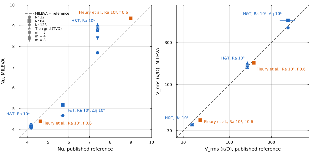
MILEVA's time-averaged Nu (left) and $V_{\mathrm{r}\mathrm{m}\mathrm{s}}$ (right) against the published value for every row of the two tables above except the two $f=0.4$ runs, which have not converged. Blue: Hernlund & Tackley (2008); orange: the Annulus column of Fleury et al. (2024). Marker shape gives the run: circle, square and diamond for Nr = 32, 64 and 128, the star for the grid TVD run, up and down triangles for the $m=4$ and $m=8$ planforms. Points on the dashed line equal the reference; the error bars on the reference axis are the published peak-to-peak spread of the time-dependent contrast-${10}^6$ case.

Exact identities

These hold for any correct discretisation, whatever any reference says. Each is asserted by a test in tests/, run by tests/run_tests.jl.

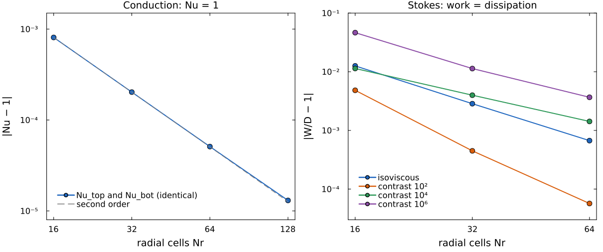
Two of these identities, recomputed by docs/scripts/plot_conservation.jl with MILEVA's own diffuse_temperature, compute_diagnostics and assemble_stokes in the spherical annulus. Left: the conducting Nusselt number converges to 1 at second order, with the top and bottom values identical. Right: $|W/D-1|$ on an exponential radial viscosity ramp shrinks under refinement at every viscosity contrast from 1 to ${10}^6$.

Conduction: Nu = 1 and Nu_top = Nu_bot

tests/test_nusselt_conduction.jl produces the conducting steady state with the diffusion solver itself (backward Euler, $\mathrm{\Delta }t\gg D^2/\kappa$) and evaluates compute_diagnostics on it. The wall flux is the one the diffusion operator uses, $k(T_{\mathrm{b}\mathrm{c}}-T_{\mathrm{w}\mathrm{a}\mathrm{l}\mathrm{l}\mathrm{c}\mathrm{e}\mathrm{l}\mathrm{l}})/(\mathrm{\Delta }r/2)$, with the Dirichlet value held at the face.

Geometry	Nr = 16	Nr = 32	Nr = 64
spherical annulus, $|\mathrm{Nu}-1|$	8.1e-4	2.0e-4	5.1e-5
cylindrical annulus, $|\mathrm{Nu}-1|$	2.5e-4	6.4e-5	1.6e-5

Second-order convergence, and ${\mathrm{Nu}}_{\mathrm{t}\mathrm{o}\mathrm{p}}={\mathrm{Nu}}_{\mathrm{b}\mathrm{o}\mathrm{t}}$ to round-off at every resolution (asserted to a relative 1e-9).

Energy budget closure

The same test takes one backward-Euler step from an arbitrary field and checks that the change of thermal energy equals the net wall power computed from the reported wall gradients:

$$\rho c_p\frac{d}{dt}\sum _c{T}_c|c|=P_{\mathrm{b}\mathrm{o}\mathrm{t}}-P_{\mathrm{t}\mathrm{o}\mathrm{p}}.$$

Measured relative residual: 2.1e-15 (spherical), 5.9e-15 (cylindrical). With uniform internal heating the applied power equals the prescribed power to 1e-12 and the residual stays at 6e-15.

tests/test_marker_energy.jl checks that one marker temperature step (projection, grid diffusion, sub-grid relaxation, hand-back) moves exactly the energy the grid solver computed, $\sum _m{w}_m\mathrm{\Delta }{T}_m=\sum _c\mathrm{\Delta }{T}_c|c|$:

Path	Relative residual
2-D spherical annulus, exact delivery	5.3e-15
2-D cylindrical annulus, exact delivery	2.6e-15
3-D Yin patch, exact delivery	5.1e-11
3-D Yin patch, production cap deliveryScaleMax = 2	7.2e-2

In the last row the cap applies at Yin-patch edge nodes, which carry half-cell marker support.

In a running model the same bookkeeping is logged every diagEvery steps as budget_resid in diagnostics.csv: the change of thermal energy against the boundary and internal power accumulated every step with the diffusion solver's own theta weighting (boundary_power, utils/diagnostics_csv.jl), normalised by the larger of the surface and internal power. A conservative run gives about zero. Measured values on the H&T runs are in the tables above (|budget_resid| ≤ 0.002 on the marker path). The grid TVD path is slightly non-conservative (+0.011), and marker reseeding is the one remaining non-conservative operation on the marker path.

Work equals dissipation (2-D)

For any Stokes solution with no-normal-flow walls the buoyancy work equals the viscous dissipation, at any viscosity field:

$$W=\int \mathbf{f}\cdot \mathbf{v}dV=\int 2\eta \dot{\mathit{\epsilon }}:\dot{\mathit{\epsilon }}dV=\int 4\eta {\dot{\epsilon }}_{II}^{2}dV=D,W/D=1.$$

Unlike rigid rotation, on which $\dot{\mathit{\epsilon }}\equiv 0$, this identity exercises the viscosity-gradient part of the operator. Measured on a fixed analytic load, Nr = 24 / 48 / 96:

Contrast	$W/D$
1	0.995 / 0.999 / 1.000
10	0.996 / 0.999 / 1.000
${10}^3$	1.002 / 1.001 / 1.001
${10}^6$	1.019 / 1.006 / 1.003

tests/test_annulus_operator.jl asserts $W>0$, $D>0$ and $|W/D-1|<0.05$ in the spherical annulus on an exponential radial viscosity ramp. Measured at Nr = 32:

Contrast	1	${10}^2$	${10}^4$	${10}^6$	${10}^8$
$W/D$	0.9971	0.9996	1.0040	1.0113	1.0211

At ${10}^8$, $|W/D-1|$ falls from 0.021 (Nr = 32) to 0.0063 (Nr = 64).

Rigid rotation is annihilated (2-D)

Rigid rotation has $\dot{\mathit{\epsilon }}\equiv 0$, so it is an exact null mode of $\mathrm{\nabla }\cdot (2\eta \dot{\mathit{\epsilon }})$ in every geometry. The operator returns a relative residual of 1.5e-16, 1.4e-16 and 2.3e-16 at Nr = 12, 24, 48 in the spherical annulus. tests/test_annulus_operator.jl asserts a residual below 1e-12.

Other exact properties in the suite

Test	Property
tests/test_conduction_conservation.jl	Radial conduction is a flux difference that telescopes over a column; ALA diffusivity profile and conductive baselines in both geometries.
tests/test_quiescence.jl	A model with no lateral structure, no boundary contrast and no sources does nothing: temperature stays uniform, velocity at round-off, energy unchanged.
tests/test_advection_consistency.jl	3-D temperature advection: a uniform field is stationary, a divergence-free radial flow preserves a constant, no overshoot of global bounds, TVD less diffusive than upwind.
tests/test_energy_consistency.jl	Dissipation equals buoyancy work, converges under refinement and survives production-like viscosity fields; the two O(Di) terms of the ALA energy equation balance on the flow they describe.
tests/test_solution_convergence.jl	A stationary Stokes solve settles under refinement.
tests/test_melt_conservation.jl	Melt mass, composition and energy bookkeeping close.

3-D operator checks

Gradient and divergence are adjoint (G = −Bᵀ)

The finite-volume 3-D assembly (assemble_stokes_3d) makes the discrete gradient the negative transpose of the discrete divergence. Measured on an 8 × 8 × 24 Yin patch, restricting to interior velocity rows (excluding the Dirichlet wall rows and the pinned pressure cell):

Block	$\Vert G+B^{\mathsf{T}}\Vert$
all velocity rows	0 exactly
$V_r$	0
$V_{\theta }$	0
$V_{\varphi }$	0

verify_g_minus_bt(L, meta) in solvers/stokes_assembly_3d.jl compares the full blocks, Dirichlet and pin rows included, and therefore returns about 0.40 on the same patch; that number does not measure the interior operator.

Work equals dissipation (3-D)

Same identity, Yin-Yang patch with a radial viscosity ramp, Nr = 8 / 12 / 16:

Contrast	Nr = 8	Nr = 12	Nr = 16
1	0.9961	1.0026	1.0029
${10}^2$	0.9880	0.9952	0.9985
${10}^4$	0.9909	0.9921	0.9953
${10}^6$	0.9812	0.9813	0.9841

Every contrast improves under refinement. tests/test_stokes_3d_variable_eta.jl asserts $|W/D-1|<0.05$ at Nr = 8 and 12 for contrasts 1 and ${10}^4$, and that refinement does not make it worse; it measures 0.9961 / 1.0026 and 0.9910 / 0.9922, matching the table.

Rigid rotation (3-D)

With cfg.useCurvatureTerms = true (the default, the full spherical deviatoric stress) the rigid-rotation residual is 2.0e-16 / 2.5e-16 / 2.5e-16 at Nr = 8 / 12 / 16, independent of the viscosity field. tests/test_spherical_operator_nullmode.jl pins both branches.

Yin-Yang geometry

tests/test_yy_rotation_vs_ks2004.jl checks the vector rotation between the patches against Kageyama & Sato (2004), Eqs. 22-23; agreement is to machine precision. This is verification against a published analytic formula.

The 3-D checks on this page are exact identities of the operator and the Yin-Yang rotation; a comparison of Nu and $V_{\mathrm{r}\mathrm{m}\mathrm{s}}$ with a published 3-D shell benchmark is not listed yet. How the patches are coupled across their seam is described on the Yin-Yang grid page.

Regression tests and smoke tests

Test	What it compares	Kind
tests/test_stokes.jl	MUMPS against UMFPACK on the same assembled system.	regression (both solve the same matrix, so it cannot detect a wrong operator)
tests/test_2d_vcycle_scgs.jl	2-D multigrid against the MUMPS solution.	regression
tests/test_assembly_3d_mirror.jl	Serial and distributed 3-D assemblies give the same matrix and right-hand side to 1e-13.	regression
tests/test_config_matrix.jl, tests/test_config_timeloop.jl	Every geometry, mode and advertised flag constructs and survives the time loop.	smoke
tests/test_full_feature_smoke.jl	Every 3-D physics flag survives two steps.	smoke
tests/smoke_stokes_3d_mg.jl	One 3-D multigrid Stokes solve (default target of bin/mileva test).	smoke
tests/test_mpi_*.jl	MPI tiers; need mpiexec, not run by tests/run_tests.jl.	regression

Run the suite with

JULIA_NUM_THREADS=4 julia --project=. tests/run_tests.jl

It reports 1404 passes, 0 failures, 0 errors in about five minutes.

Scripts outside the runner: tests/test_amr_full.jl (its baseline iteration count of 40 predates the current 3-D solver, which converges in 31), and tests/test_mdpi_eta_contrast.jl, tests/test_vcycle_visc_contrast_sweep.jl, tests/test_arrhenius_viscosity.jl, tests/test_fk_viscosity.jl and the smoke_* chunk scripts, which print their results rather than asserting them.

Related pages: Parameter reference, Function reference.