Rheology

Rheology is the relation between the stress a material carries and the rate at which it deforms. In a mantle-convection model it enters through one field, the viscosity $\eta$, and that field decides more about the outcome than almost any other input. It sets whether the surface moves as plates, as a single stagnant lid or in episodic overturns, how thick and how cold the lithosphere becomes, and how fast the interior loses its heat. This page first explains the physics behind the viscosity laws, then how MILEVA evaluates them.

Physical background

Why solid rock flows

The mantle is solid. It transmits shear waves and, over seconds to years, it deforms elastically. Over millions of years it flows, because at temperatures above roughly half its melting temperature a crystalline rock deforms by thermally activated creep. Atoms diffuse through and around the grains, and lattice defects (dislocations) glide and climb through the crystals. Each of these processes produces a strain rate that grows with stress and very steeply with temperature (Karato 2008; Turcotte & Schubert 2014).

The time scale that separates the elastic from the viscous response is the Maxwell time, $t_M=\eta /G$. With a viscosity of ${10}^{21}$ Pa s and a shear modulus of about 70 GPa, the upper-mantle value of the preliminary reference Earth model (Dziewonski & Anderson 1981), $t_M$ is about 450 years. Convection evolves over tens of millions of years, so the interior can be treated as a viscous fluid, and elasticity only matters in the cold lid (see Visco-elasto-plasticity).

A creeping rock is described by an effective viscosity, the ratio of the deviatoric stress to twice the strain rate,

$${\tau }_{ij}=2\eta {\dot{\epsilon }}_{ij},\eta =\frac{{\tau }_{II}}{2{\dot{\epsilon }}_{II}},$$

where ${\tau }_{II}$ and ${\dot{\epsilon }}_{II}$ are the second invariants of the deviatoric stress and strain-rate tensors. For a Newtonian mechanism $\eta$ does not depend on the stress; for a non-Newtonian one it does, and the "viscosity" is simply the value that reproduces the current stress at the current strain rate. With $\eta ={10}^{21}$ Pa s and a strain rate of ${10}^{-15}$ s⁻¹ (a plate speed of 5 cm/yr sheared over 1000 km gives $1.6\times {10}^{-15}$ s⁻¹) the stress is $2\eta {\dot{\epsilon }}_{II}=2$ MPa, the order of magnitude of convective stresses in the interior.

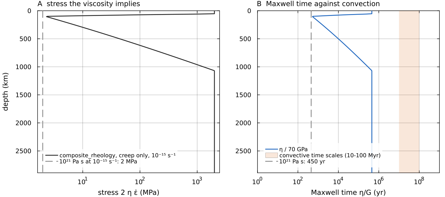
Creep viscosity from composite_rheology (yield branch switched off, default clamps) along the code's geotherm, an adiabat of 1600 K potential temperature below a 100 km conductive lid, at ${10}^{-15}$ s⁻¹. Left: the stress $2\eta {\dot{\epsilon }}_{II}$ it implies. Right: the Maxwell time $\eta /G$ with $G=70$ GPa. Even the cells held at the upper clamp of ${10}^{24}$ Pa s relax within about 450 kyr, far below the 10 to 100 Myr of convection. Script: docs/scripts/fig_rheology_sections.jl.

Deformation mechanisms

Laboratory experiments on olivine, the dominant upper-mantle mineral, identify several creep mechanisms (Karato & Wu 1993; Hirth & Kohlstedt 2003). They differ in how the strain rate depends on stress $\tau$ and grain size $d$:

mechanism	strain rate scales as	viscosity	where it matters
diffusion creep	$\tau d^{-m}$, $m\approx 2$-3	Newtonian, grain-size sensitive	hot mantle, small grains, low stress
dislocation creep	${\tau }^n$, $n\approx 3$-3.5	strain-rate weakening, grain-size insensitive	higher stress, larger grains, upper mantle and lid base
grain-boundary sliding	${\tau }^n{d}^{-m}$	both stress and grain-size sensitive	intermediate conditions
Peierls (low-temperature) plasticity	exponential in $\tau$	very strongly stress dependent	cold lithosphere at high stress
frictional sliding and fracture	stress set by pressure, not by rate	perfectly plastic	the brittle upper lithosphere

All the thermally activated mechanisms share an Arrhenius dependence $\exp [-(E+PV)/RT]$, with activation energy $E$ and activation volume $V$. For dry olivine $E$ is about 300 to 375 kJ/mol in diffusion creep and 530 to 540 kJ/mol in dislocation creep, with a stress exponent of 3.5 (Karato & Wu 1993; Hirth & Kohlstedt 2003); the values each preset carries are listed on the Flow laws page.

Mechanisms that operate side by side in the same grains act in parallel. Each accommodates part of the deformation at the same stress, so their strain rates add, and at a common stress their viscosities combine harmonically, $1/\eta =\sum _{k}1/{\eta }_k$. The weakest mechanism carries most of the strain. Which one that is depends on stress, grain size and temperature, and a deformation-mechanism map is a plot of exactly this competition (Karato 2008). Karato & Wu (1993) concluded that the upper mantle lies close to the boundary between diffusion and dislocation creep, which is why a composite law that keeps both is the usual choice.

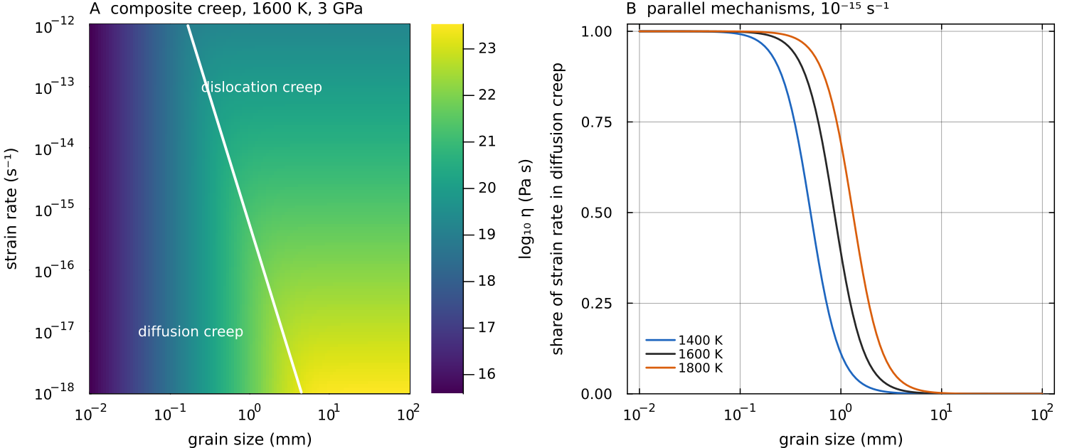
The default reference-viscosity creep laws of composite_rheology at 1600 K and 3 GPa, with the grain size entering diffusion creep (cfg.evolveGrainSize = true). Left: the viscosity of the parallel combination; the white line is where diffusion and dislocation creep are equally strong. Right: the fraction of the strain rate carried by diffusion creep, ${\eta }_{\text{duct}}/{\eta }_{\text{diff}}$, at ${10}^{-15}$ s⁻¹. At 1600 K the two mechanisms share the deformation equally near 1 mm grains, and a hotter mantle moves the boundary to larger grains. Script: docs/scripts/fig_rheology_sections.jl.

Near the surface a different limit applies. Cold rock cannot creep fast enough, and it fails by fracture and frictional sliding instead, at a stress that rises with the confining pressure and hardly depends on the strain rate. Laboratory friction coefficients of 0.6 to 0.85 hold for most rock types (Byerlee 1978). The strength of the lithosphere at any depth is the smaller of the brittle and the ductile strength, the "strength envelope" reviewed by Kohlstedt, Evans & Mackwell (1995). Convection models need effective friction coefficients well below Byerlee's values to break the lid into plates (Moresi & Solomatov 1998; Tackley 2000), which is commonly attributed to pore-fluid pressure and to weak, pre-existing faults.

How strongly the viscosity varies

The Arrhenius factor makes temperature the dominant control. Differentiating it gives $\partial \ln \eta /\partial T=-E/(R{T}^2)$, so the temperature change that alters $\eta$ by a factor 10 is $\ln 10R{T}^2/E$. The numbers below are evaluated with MILEVA's default composite-path parameters (table further down), at the reference temperature of 1600 K unless stated:

change	diffusion creep ($E$ = 300 kJ/mol, $V$ = 6 cm³/mol)	dislocation creep ($E$ = 540 kJ/mol, $V$ = 14 cm³/mol, $n$ = 3.5)
temperature change for a factor 10	163 K	318 K (the exponent is divided by $n$)
cooling from 1600 K to 1000 K, at $P=0$	$\times 7.5\times {10}^5$	$\times 1.1\times {10}^3$ at fixed strain rate
pressure from 0 to 5 GPa	$\times 9.5$	$\times 4.5$
strain rate $\times 10$	no change	$\times 0.19$
grain size $\times 2$ ($m$ = 3)	$\times 8$	no change

A cold lid is therefore many orders of magnitude stiffer than the interior. A convenient measure of this sensitivity is the Frank-Kamenetskii parameter $\theta =E\mathrm{\Delta }T/(R{T}_i^2)$, with $\mathrm{\Delta }T$ the temperature drop across the layer and $T_i$ the interior temperature; $e^{\theta }$ approximates the viscosity contrast across the layer. As the contrast grows, convection passes from a small-contrast regime through a sluggish-lid regime to the stagnant-lid regime, in which the cold top boundary layer stops taking part in the flow and the interior convects beneath it; Solomatov (1995) places the stagnant-lid regime above a contrast of order ${10}^4$. Whether a planet has a stagnant lid, plates or episodic overturns is then decided by the competition between this temperature-dependent stiffening and the yield stress of the lid (Moresi & Solomatov 1998). With power-law creep the temperature and pressure terms are divided by $n$ at a fixed strain rate, as the right-hand column shows, so the same activation energy produces a smaller contrast; Christensen (1984) studied convection with this combined temperature, pressure and stress dependence.

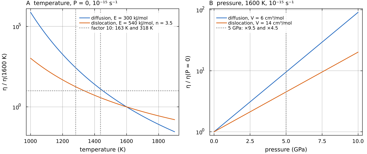
The default diffusion and dislocation laws of composite_rheology, each alone and normalised to its value at the reference state, at a fixed strain rate of ${10}^{-15}$ s⁻¹. Left: temperature at zero pressure; the dotted lines mark the 163 K and 318 K of cooling that raise each viscosity tenfold. Right: pressure at 1600 K; at 5 GPa the factors are 9.5 and 4.5, as in the table. Script: docs/scripts/fig_rheology_sections.jl.

Typical values

quantity	value	source
Earth, average upper-mantle viscosity	${10}^{20}$ to ${10}^{21}$ Pa s, increasing substantially into the lower mantle	Mitrovica & Forte (2004)
Venus, interior viscosity inferred from stagnant-lid scaling	${10}^{20}$ to ${10}^{21}$ Pa s	Solomatov & Moresi (1996)
mantle strain rates	of order ${10}^{-15}$ s⁻¹	estimate above
rock friction coefficient	0.6 to 0.85	Byerlee (1978)
olivine activation energy	300 to 540 kJ/mol	Karato & Wu (1993); Hirth & Kohlstedt (2003)

Venus has no plate tectonics today, and its surface is dry. Mackwell, Zimmerman & Kohlstedt (1998) found dry diabase, a proxy for the Venus crust, to be much stronger than earlier wet-rock data suggested, which favours a strong lid; this is why the crustal presets of the Flow laws page include their law.

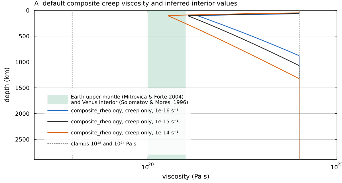
Creep viscosity of composite_rheology with default parameters (yield branch off) on the geotherm of the figures above, at three strain rates, against the ${10}^{20}$ to ${10}^{21}$ Pa s inferred for the Earth's upper mantle and the Venus interior. Without layered activation parameters the pressure term makes the viscosity grow with depth until it reaches the upper clamp below about 900 to 1300 km. The defaults are generic values, not a calibration to either planet, so a planetary run sets them against the inferred range. Script: docs/scripts/fig_rheology_sections.jl.

How MILEVA builds the viscosity

The viscosity $\eta$ that enters the Stokes operator is built once per time step (and again inside the nonlinear iteration) in step (2) of the time loop in main_SphCon.jl. There are two paths, chosen by cfg.useCompositeRheology:

path	cfg.useCompositeRheology	entry point	depends on
simple	false (default)	compute_viscosity (physics/compute_viscosity.jl), optionally overwritten by frank_kamenetskii_viscosity! (utils/fk_viscosity.jl)	$T$, depth layer, composition multipliers
composite	true	composite_rheology (physics/composite_rheology.jl)	$T$, $P$, ${\dot{\epsilon }}_{II}$, grain size, composition, accumulated strain

Both end with the clamp $\eta \in [{\eta }_{\text{min}},{\eta }_{\text{max}}]$ (cfg.eta_min = 1e18, cfg.eta_max = 1e24 Pa s by default). Optional modifiers (visco-elasto-plasticity, damage) are then applied on top, in that order.

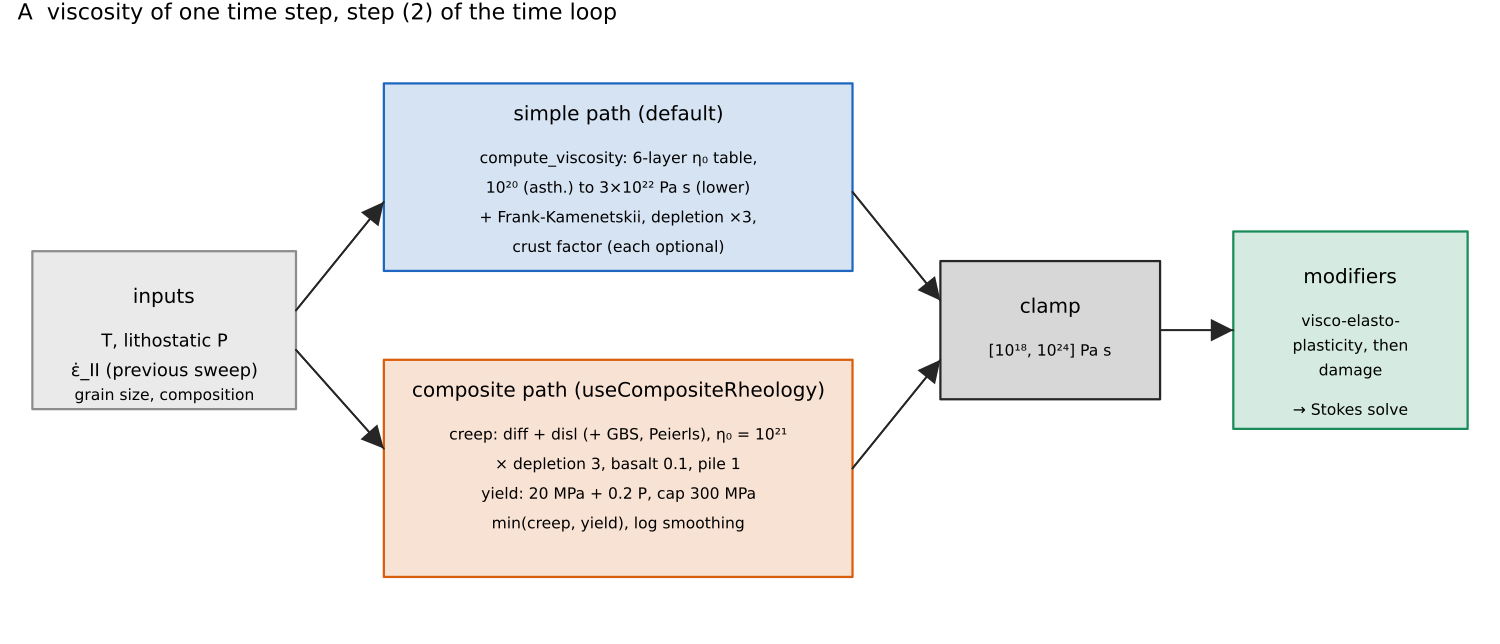
The two paths that build the viscosity in step (2) of the time loop, with the default values each stage uses. Schematic; the numbers are the defaults of MaterialProperties and SimConfig. Script: docs/scripts/fig_rheology_sections.jl.

The strain-rate invariant used throughout is

$${\dot{\epsilon }}_{II}=\sqrt{\frac{1}{2}({\dot{\epsilon }}_{rr}^2+{\dot{\epsilon }}_{\theta \theta }^2+{\dot{\epsilon }}_{\varphi \varphi }^2)+{\dot{\epsilon }}_{r\theta }^2}$$

in 2-D (the ${\dot{\epsilon }}_{\varphi \varphi }=V_r/r$ term only in the spherical annulus) and the full six-component form in 3-D (compute_strain_rate, utils/compute_strain_rate.jl). The 2-D routine returns a raw and a spatially smoothed invariant; the rheology uses the smoothed one, the dissipation diagnostic the raw one. compute_strain_rate guards the square root with a floor of ${10}^{-30}$ s${}^{-1}$ and composite_rheology floors ${\dot{\epsilon }}_{II}$ at ${10}^{-20}$ s${}^{-1}$, both far below mantle strain rates.

Simple path: layered Arrhenius

compute_viscosity evaluates a pressure-scaled Arrhenius law on a six-layer prefactor table:

$$\eta (T,r)={\eta }_0^{(\ell )}\exp [(E^{\ast }+V^{\ast }P)(\frac{1}{T}-\frac{1}{T_{\text{ref}}})],P={\rho }_{0}g(R_{\text{out}}-r),$$

where $E^{\ast }$ = mat.E_act_scale and $V^{\ast }$ = mat.V_act_scale are in kelvin and kelvin per pascal (an activation energy and volume divided by the gas constant), $T_{\text{ref}}$ = mat.T_ref, and $T$ is floored at 300 K. The layer $\ell$ comes from get_layer(mat, r) (config/MaterialProperties.jl):

layer	radius range	prefactor field	default (Pa s)
1, D″	$r\le$ R_Dprime	Dprime_eta0	${10}^{22}$
2, lower mantle	$\le$ R_lower	lower_eta0	$3\times {10}^{22}$
3, transition zone	$\le$ R_trans	trans_eta0	${10}^{22}$
4, upper mantle	$\le$ R_upper	upper_eta0	${10}^{21}$
5, asthenosphere	$\le$ R_asth	asth_eta0	${10}^{20}$
6, lithosphere	above	lith_eta0	${10}^{23}$

The layer radii default to Earth values and must be set for another planet. Setting all six prefactors equal and $E^{\ast }=0$ gives an isoviscous mantle, which is how the Hernlund & Tackley benchmark driver configures its isoviscous cases.

The 3-D method of compute_viscosity uses the same table with the exponent $E^{\ast }(1/T-1/T_{\text{ref}})$, without the mat.V_act_scale term.

This path is a prescribed, Newtonian viscosity. It depends on temperature and depth but not on stress, grain size or strain history, which makes it the natural choice for benchmarks and for isolating thermal effects. Because $E^{\ast }$ is an activation energy divided by the gas constant, a mantle-like 300 kJ/mol corresponds to $E^{\ast }\approx 3.6\times {10}^4$ K. The default mat.E_act_scale = 200 K is far smaller and gives an almost depth-layered viscosity; between 1600 K and 1000 K it changes $\eta$ by only a factor 1.08. A run that relies on temperature-dependent stiffening on this path must therefore set $E^{\ast }$ (or use the Frank-Kamenetskii form below) explicitly.

After compute_viscosity, the simple path applies, in order:

1. Frank-Kamenetskii (cfg.useFrankKamenetskii), which overwrites $\eta$ entirely with one of two forms selected by cfg.fkForm:

$$\text{"linearized":}\eta ={\eta }_{\text{ref}}\exp [\frac{E}{1+T/T_{\text{ref}}}-\frac{E}{2}],\text{"simple":}\eta ={\eta }_{\text{ref}}\exp [-{\theta }_{FK}\frac{T-T_{\text{surf}}}{T_{\text{cmb}}-T_{\text{surf}}}],$$

with fk_eta_ref, fk_E, fk_T_ref and fk_theta. Both are approximations to the Arrhenius law that keep the viscosity contrast bounded and controllable. The simple form is the exponential approximation named after Frank-Kamenetskii, linear in $T$ in the exponent. The linearized form has an exponent proportional to $1/(1+T/T_{\text{ref}})$, which resembles the Arrhenius $1/T$ but stays finite as $T\to 0$, so the viscosity contrast is at most $e^{E/2}$ on either side of ${\eta }_{\text{ref}}$. The simple form gives a viscosity contrast $e^{{\theta }_{FK}}$ across the layer; the Hernlund & Tackley variable-viscosity cases use it with ${\theta }_{FK}=\ln {10}^6=13.8155$.

2. Depletion stiffening (cfg.useDepletionStiffening): $\eta \leftarrow \eta [1+(\xi -1)min(C_{\text{dep}}/F_{\text{max}},1)]$ with $\xi$ = mat.harzburgite_eta_factor (default 3) and $F_{\text{max}}$ = cfg.fertileFraction (default 0.30), the same factor the composite path applies.

3. Crust factor (2-D, cfg.crustViscosityFactor $\ne 1$): $\eta \leftarrow \eta [1+(f_c-1)X_{\text{crust}}]$, with the crust fraction $X_{\text{crust}}$ defined in Buoyancy and composition.

4. Yield cap (cfg.useSimpleYield, exercised in 2-D only): simple_yield! in physics/compute_viscosity.jl caps the stress at the Drucker-Prager yield stress of the composite path, ${\tau }_y=min(C+\mu P,{\tau }_{\text{max}})$ with the same MaterialProperties fields, by $\eta \leftarrow min(\eta ,{\tau }_y/2{\dot{\epsilon }}_{II})$. Unlike the composite path it acts at every temperature (cfg.yieldMinT is not applied). The viscosity is then nonlinear, so the time loop iterates it with the solve (Nonlinear iteration); the stagnant-lid example uses it with a depth-independent ${\tau }_y$. validate! refuses it together with useCompositeRheology or a radial viscosity file.

Each step re-clamps to $[{\eta }_{\text{min}},{\eta }_{\text{max}}]$.

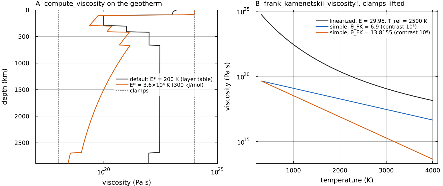
Left: compute_viscosity on a 300-cell column of the default shell, on the geotherm used above. With the default $E^{\ast }=200$ K the six-layer prefactor table sets the profile; with $E^{\ast }=3.6\times {10}^4$ K (300 kJ/mol) the cold lid reaches the upper clamp and the hot deep mantle approaches the lower one. Right: frank_kamenetskii_viscosity! between the default surface and core-mantle-boundary temperatures (300 and 4000 K) with the clamps lifted, for the default linearized form and the simple form at two values of ${\theta }_{FK}$. Script: docs/scripts/fig_rheology_sections.jl.

arrhenius_viscosity! (utils/arrhenius_viscosity.jl, cfg.useArrhenius) and apply_660km_jump! (utils/viscosity_jumps.jl) are standalone utilities for drivers and tests; main_SphCon applies the Arrhenius law above, and cfg.use660kmJump acts on the composite path (below).

Composite path

composite_rheology evaluates, in this order (the file header documents the same sequence).

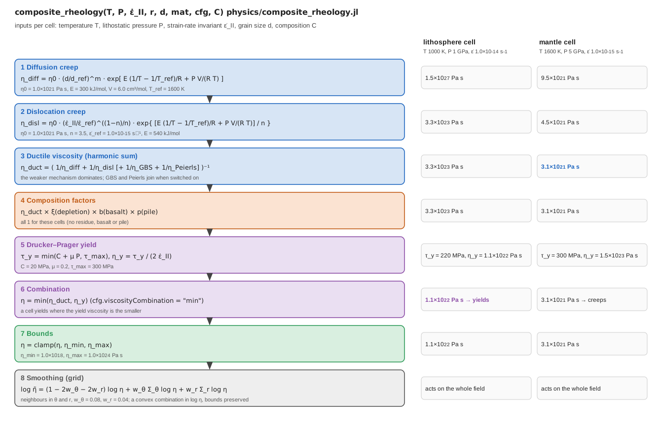
The computation for one cell, stage by stage, with the default material parameters. Right: the value each stage produces for a cold lithosphere cell (1000 K, 1 GPa, ${10}^{-14}$ s⁻¹), which yields, and a hot mantle cell (1600 K, 5 GPa, ${10}^{-15}$ s⁻¹), which creeps; the final values equal what composite_rheology returns for those cells. Script: docs/scripts/fig_rheology_pipeline.jl.

1. Ductile creep

With lithostatic pressure $P$ from mantle_pressure (the reference state of the selected compressibility mode) and $T$ floored at 300 K:

$${\eta }_{\text{diff}}={\eta }_{0,\text{diff}}(\frac{d}{d_{\text{ref}}}{)}^m\exp [\frac{E_{\text{diff}}}{R}(\frac{1}{T}-\frac{1}{T_{\text{ref}}})+\frac{P{V}_{\text{diff}}}{RT}],$$$${\eta }_{\text{disl}}={\eta }_{0,\text{disl}}(\frac{{\dot{\epsilon }}_{II}}{{\dot{\epsilon }}_{\text{ref}}}{)}^{(1-n)/n}\exp \{\frac{1}{n}[\frac{E_{\text{disl}}}{R}(\frac{1}{T}-\frac{1}{T_{\text{ref}}})+\frac{P{V}_{\text{disl}}}{RT}]\},$$$${\eta }_{\text{duct}}=(\frac{1}{{\eta }_{\text{diff}}}+\frac{1}{{\eta }_{\text{disl}}}+\frac{1}{{\eta }_{\text{GBS}}}+\frac{1}{{\eta }_{\text{P}}}{)}^{-1}.$$

Here

symbol	meaning	unit
$T$	absolute temperature of the cell, floored at 300 K	K
$P$	lithostatic pressure at the cell's depth below mat.R_surf	Pa
$R$	gas constant, cfg.R_GAS = 8.314	J mol⁻¹ K⁻¹
$E$, $V$	activation energy and activation volume of the mechanism	J mol⁻¹, m³ mol⁻¹
${\eta }_0$	reference viscosity of the mechanism	Pa s
$T_{\text{ref}}$	reference temperature at which $\eta ={\eta }_0$ (with $P=0$)	K
$d$, $d_{\text{ref}}$, $m$	grain size, reference grain size and grain-size exponent	m, m, -
${\dot{\epsilon }}_{II}$, ${\dot{\epsilon }}_{\text{ref}}$, $n$	strain-rate invariant, reference strain rate and stress exponent	s⁻¹, s⁻¹, -
${\eta }_{\text{GBS}}$, ${\eta }_{\text{P}}$	grain-boundary-sliding and Peierls viscosities, infinite unless switched on	Pa s

Where the exponents come from. These are laboratory creep laws written in a reference-viscosity form. A power law $\dot{\epsilon }=A{\tau }^n{d}^{-m}\exp [-(E+PV)/RT]$ solved for the stress and divided by $2\dot{\epsilon }$ gives

$$\eta =\frac{1}{2}{A}^{-1/n}{\dot{\epsilon }}^{(1-n)/n}{d}^{m/n}\exp [\frac{E+PV}{nRT}],$$

so a stress exponent $n$ turns into a strain-rate exponent $(1-n)/n$ and divides the Arrhenius term by $n$. Diffusion creep is the case $n=1$, for which the viscosity is Newtonian and scales with $d^m$. Instead of the prefactor $A$, MILEVA prescribes the viscosity ${\eta }_0$ that each law has at $T_{\text{ref}}$, $P=0$, $d_{\text{ref}}$ and (for dislocation creep) ${\dot{\epsilon }}_{\text{ref}}$, which is easier to choose and to compare between mechanisms. The temperature term $(1/T-1/T_{\text{ref}})$ vanishes at $T_{\text{ref}}$, while the pressure term $PV/RT$ is not referenced, so ${\eta }_0$ is a zero-pressure value. In the dislocation law the grain-size factor is absent because dislocation creep does not depend on grain size. The harmonic sum ${\eta }_{\text{duct}}$ is the parallel combination described in Deformation mechanisms, in which whichever mechanism is weakest at the cell's conditions sets the viscosity.

parameter	field	default
${\eta }_{0,\text{diff}}$, ${\eta }_{0,\text{disl}}$	mat.diff_eta0, mat.disl_eta0	${10}^{21}$ Pa s
$T_{\text{ref}}$	mat.T_ref	1600 K
$E$, $V$ diffusion, upper / lower	diff_E_upper/lower, diff_V_upper/lower	300 / 200 kJ mol${}^{-1}$, 6 / 3 cm${}^3$ mol${}^{-1}$
$E$, $V$ dislocation, upper / lower	disl_E_upper/lower, disl_V_upper/lower	540 / 300 kJ mol${}^{-1}$, 14 / 3 cm${}^3$ mol${}^{-1}$
$n$, ${\dot{\epsilon }}_{\text{ref}}$	mat.disl_n, mat.disl_eII_ref	3.5, ${10}^{-15}$ s${}^{-1}$
$m$, $d_{\text{ref}}$	mat.diff_m, mat.diff_d_ref	3, 1 mm

The lower-mantle values of $E$ and $V$ are used only when cfg.useLayeredActivationEnergy = true; otherwise the upper values apply everywhere. The grain-size factor is 1 unless cfg.evolveGrainSize is on (Grain-size evolution).

Two optional mechanisms join the harmonic sum: grain-boundary sliding (cfg.useGBS, parameters cfg.gbs_A, gbs_n, gbs_m and mat.gbs_E_upper/lower) and Peierls low-temperature plasticity (cfg.usePeierlsCreep, active only where $T<1100$ K; the law is mat.flowlaw_peierls, Mei et al. 2010 by default). Both default off.

Published flow laws

Instead of the reference-viscosity laws above, the diffusion and dislocation creep of the mantle, a crustal law where there is basalt, and the Peierls law can be taken from published laboratory experiments (Hirth & Kohlstedt 2003, Karato & Wu 1993, Mackwell et al. 1998, Rybacki & Dresen 2000 and others), by name. See Flow laws.

Lower-mantle offset. With cfg.use660kmJump = true, every creep law below cfg.depth660km is multiplied by a prefactor (lower_mantle_creep_prefactors) that divides out the jump the $E$/$V$ switch itself produces at the interface (evaluated at the horizontal-mean $T$ and $P$ of the two rows that straddle it, lower_mantle_interface_TP) and multiplies by cfg.eta660kmFactor. The viscosity ratio across the interface is then exactly eta660kmFactor at the interface conditions, and the $E$/$V$ switch and the yield-parameter switch are moved to cfg.depth660km rather than mat.R_lower.

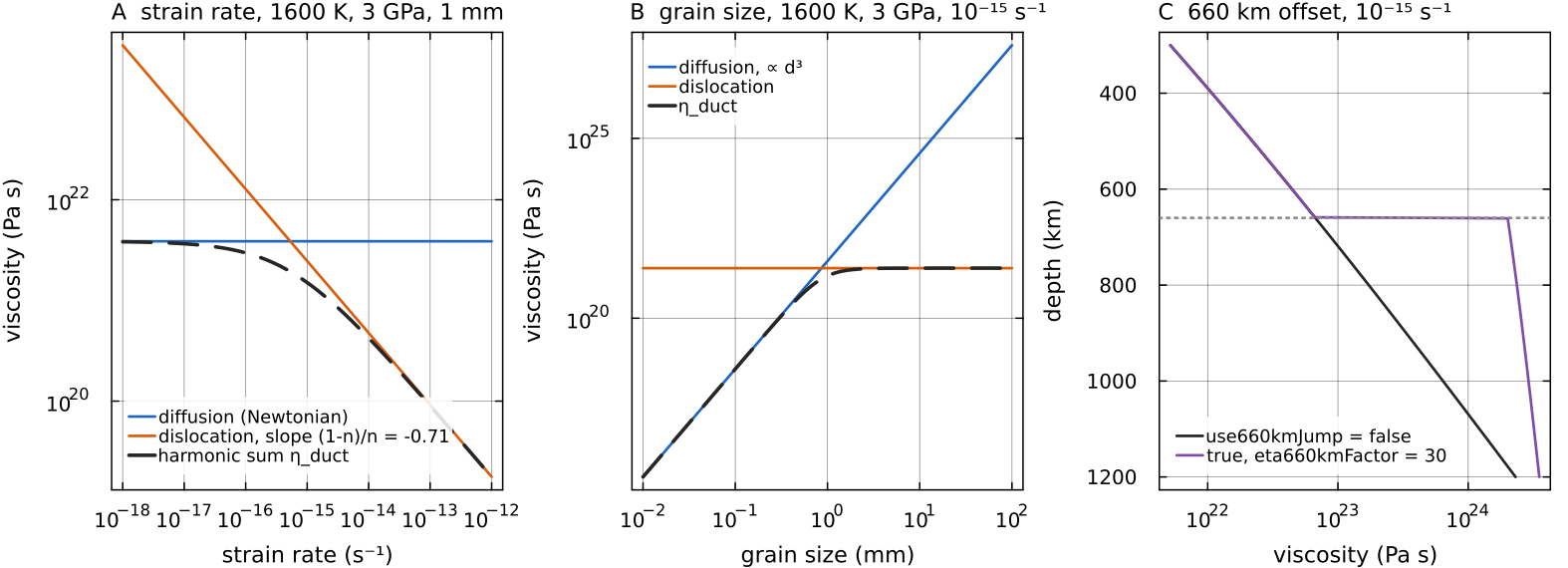
The ductile branch of composite_rheology with default parameters, yield off and clamps lifted. Left: diffusion creep is independent of the strain rate and dislocation creep falls with slope $(1-n)/n=-0.71$; the harmonic sum follows the weaker law. Middle: diffusion creep scales as $d^3$ (with cfg.evolveGrainSize = true), and the sum saturates at the dislocation value for large grains. Right: the geotherm between 300 and 1200 km with cfg.use660kmJump and cfg.useLayeredActivationEnergy on; the viscosity rises by exactly eta660kmFactor = 30 across the interface (30.3 between the two rows that straddle it). Script: docs/scripts/fig_rheology_sections.jl.

2. Composition factors

Applied to ${\eta }_{\text{duct}}$ only:

$${\eta }_{\text{duct}}\leftarrow {\eta }_{\text{duct}}[1+(\xi -1)min(C_{\text{dep}}/F_{\text{max}},1)][1+(b-1)C_{\text{bas}}][1+(p-1)C_{\text{pile}}],$$

with $\xi$ = mat.harzburgite_eta_factor (3), $b$ = mat.basalt_eta_factor (0.1) and $p$ = mat.tcpile_eta_factor (1). $C_{\text{dep}}$, $C_{\text{bas}}$ and $C_{\text{pile}}$ are the marker fields projected to cells (the previous step's values; see Melting and crust production). With cfg.depletionStiffensYield = true the depletion factor also multiplies the yield viscosity.

The three factors stand for three materials whose creep strength differs from that of fertile peridotite. Melt extraction removes water and the most fusible components, and the dry, depleted residue (harzburgite) is expected to be stiffer (Hirth & Kohlstedt 1996); $\xi$ is its viscosity ratio at full depletion, reached when $C_{\text{dep}}$ equals the fusible fraction $F_{\text{max}}$, so a partly depleted cell is stiffened in proportion to how far its melting has gone. Basalt and the thermochemical pile material enter in proportion to their fractions. Each factor is linear in its fraction and equals 1 for pure fertile mantle; this is a simple mixing rule, chosen for transparency, rather than a law derived for a two-phase aggregate. When a crustal flow law is selected (mat.flowlaw_crust_diffusion or mat.flowlaw_crust_dislocation), it replaces the basalt factor $b$, and the code then blends the mantle and crustal viscosities in $\log \eta$ by the basalt fraction (see Flow laws).

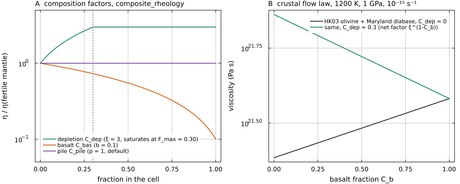
Left: the factor composite_rheology applies to the ductile viscosity of a mantle cell (1600 K, 3 GPa, ${10}^{-15}$ s⁻¹) as each composition field goes from 0 to 1 with the others at zero. Depletion stiffens linearly in $C_{\text{dep}}/F_{\text{max}}$ and saturates at $\xi =3$ once $C_{\text{dep}}$ reaches 0.30; basalt softens to $b=0.1$; the pile factor is 1 by default. Right: with published flow laws (Hirth & Kohlstedt 2003 dry olivine, Mackwell et al. 1998 Maryland diabase for the crust) the viscosity is blended in $\log \eta$, and depletion acts on the mantle fraction only. Script: docs/scripts/fig_rheology_sections.jl.

3. Drucker-Prager yield

$${\tau }_Y=min[max(C_{\text{eff}}+\mu P,0),{\tau }_{\text{max}}],{\eta }_Y=\frac{{\tau }_Y}{2{\dot{\epsilon }}_{II}},$$

with cohesion mat.cohesion_upper/lower (20 / 60 MPa), friction coefficient mat.friction_upper/lower (0.2 / 0.3) and cap mat.maxYieldStress (300 MPa). Where $T<$ cfg.yieldMinT (default 0, i.e. nowhere) the yield branch is switched off (${\eta }_Y=\mathrm{\infty }$). Setting cohesion and cap to Inf removes yielding altogether.

Continent material can carry its own law: when mat.continent_cohesion or mat.continent_friction is set (both default to NaN, which keeps the layer's values), the cohesion and friction of a cell are mixed linearly in its continent fraction $c_c$,

$$C_0\leftarrow (1-c_c)C_0+c_c{C}_c,\mu \leftarrow (1-c_c)\mu +c_c{\mu }_c,$$

so the yield stress is the volume-fraction average of the two, the same rule the continent viscosity factor follows.

The yield viscosity ${\eta }_Y$ is the viscosity at which a cell deforming at its current strain rate carries exactly the yield stress. Wherever ${\eta }_Y$ is the smaller branch, the stress in the cell is therefore held at ${\tau }_Y$ and any further loading goes into faster deformation rather than higher stress, which is the viscous representation of a rock that has failed. The yield stress grows with pressure through the friction coefficient $\mu$, like the frictional strength of Byerlee (1978), and the cap ${\tau }_{\text{max}}$ limits it at depth, where ductile creep takes over in reality. The default friction coefficients (0.2 and 0.3) lie well below Byerlee's laboratory range, in line with the reduced values that convection models use to obtain a mobile lid (Moresi & Solomatov 1998). As an illustration, at 30 km depth with $\rho =3300$ kg/m³ and $g=9.8$ m/s² the pressure is about 1 GPa and the default upper-mantle law gives ${\tau }_Y=20+0.2\times 970\approx 210$ MPa.

With cfg.useFullPlasticity = true the cohesion weakens with the accumulated plastic strain ${\epsilon }_{\text{acc}}$ carried on markers:

$$C_{\text{eff}}=C_0[1-W(1-\frac{1}{f_{sw}})],W=\mathrm{clamp}(\frac{{\epsilon }_{\text{acc}}-{\epsilon }_1}{{\epsilon }_2-{\epsilon }_1},0,1),$$

with $f_{sw}$ = cfg.strainWeakeningFactor (default 1, no weakening) and ${\epsilon }_{1,2}$ = cfg.strainWeakeningE1/E2 (0.5, 1.5). The driver adds ${\dot{\epsilon }}_{II}\mathrm{\Delta }t$ to each marker's eps_acc every step when the flag is on (see Damage, softening and healing).

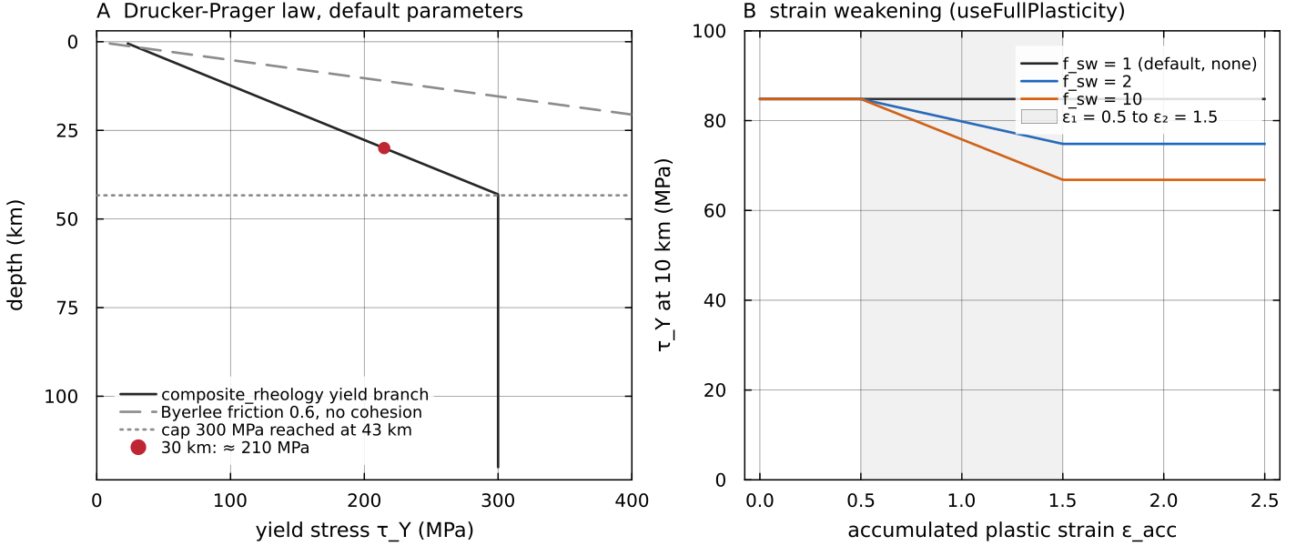
Left: the yield stress of composite_rheology's Drucker-Prager branch ($2{\eta }_Y{\dot{\epsilon }}_{II}$ with the creep laws switched off) against depth, with the default upper-mantle parameters and the lithostatic pressure of mantle_pressure. It grows by about 6.5 MPa per km, reaches 210 MPa at 30 km and the 300 MPa cap at 43 km; Byerlee's friction of 0.6 without cohesion is shown for comparison. Right: with cfg.useFullPlasticity = true the cohesion weakens between ${\epsilon }_1=0.5$ and ${\epsilon }_2=1.5$, for three values of cfg.strainWeakeningFactor; at 10 km only the 20 MPa cohesion is reduced, the pressure term is not. Script: docs/scripts/fig_rheology_sections.jl.

4. Combination, clamp and smoothing

cfg.viscosityCombination selects $\eta =min({\eta }_{\text{duct}},{\eta }_Y)$ ("min", default, the form of Tian et al. 2023 Eq. 6) or the harmonic mean $1/(1/{\eta }_{\text{duct}}+1/{\eta }_Y)$ ("harmonic"). The result is clamped to $[{\eta }_{\text{min}},{\eta }_{\text{max}}]$ and then smoothed once in ${\log }_{10}\eta$:

$$\log {\tilde{\eta }}_{ij}=(1-2w_{\theta }-2w_r)\log {\eta }_{ij}+w_{\theta }(\log {\eta }_{i,j+1}+\log {\eta }_{i,j-1})+w_r(\log {\eta }_{i+1,j}+\log {\eta }_{i-1,j}),$$

with $w_{\theta }=0.08$ (periodic) and $w_r=0.04$ (one-sided at the walls) in 2-D, and a $\frac{1}{4}$-$\frac{1}{2}$-$\frac{1}{4}$ stencil along $\theta$ only in 3-D (_smooth_viscosity). Being a convex combination in log space, it preserves the clamp bounds.

The "min" rule is the strength-envelope picture of Kohlstedt, Evans & Mackwell (1995). A cell deforms by whichever mode, creep or yielding, needs the lower stress at its strain rate, and the switch between the two is sharp. The harmonic mean treats the two branches as acting in parallel; it gives a smooth transition and, where the branches are equal, a viscosity half that of the "min" rule.

The bounds and the smoothing are numerical measures rather than physics. The clamp limits the viscosity contrast the Stokes solver has to handle; a cold lid in nature can be many more orders of magnitude stiffer than ${\eta }_{\text{max}}$, so a run whose lid sits on the upper bound should be checked for sensitivity to it. The smoothing damps cell-to-cell jumps in $\log \eta$, such as those where the yield branch switches on in isolated cells.

The yield law is nonlinear

The yield viscosity ${\eta }_Y\propto {\dot{\epsilon }}_{II}^{-1}$, so the time loop iterates viscosity, solve and strain rate within the step on the composite path (see Nonlinear iteration). Keep cfg.picardMax at its automatic value or larger for any run with a finite yield stress. Inside the sweeps composite_rheology and the damage factor are reapplied; the visco-elasto-plastic reduction and the antisqueeze correction act on the first sweep.

cfg.useDruckerPrager and the dp_* fields belong to a separate helper, utils/drucker_prager.jl, used outside the time loop; validate!(cfg) refuses useDruckerPrager = true and points to the material fields above.

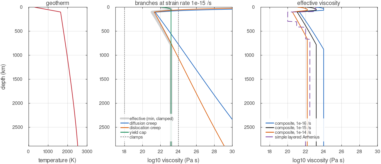
Viscosity along a geotherm (the code's adiabat at 1600 K potential temperature below a 100 km conductive lid), from composite_rheology with default parameters. Middle: each branch alone and the effective viscosity, the minimum of the branches inside the clamps; below about 700 km the default 300 MPa yield cap sets the value at this strain rate. Right: the effective viscosity at three strain rates, and the simple layered Arrhenius law of compute_viscosity on the same temperatures.

Optional modifiers

flag	file, function	what it does	details
cfg.useViscoelastoplastic	physics/viscoelastoplastic.jl, viscoelastoplastic	Maxwell viscosity with a Drucker-Prager cap	Visco-elasto-plasticity
cfg.useDamage	physics/damage.jl, evolve_damage!, apply_damage_to_viscosity!	grid damage with healing, scales the viscosity	Damage, softening and healing
cfg.evolveGrainSize	physics/evolve_grain_size.jl, evolve_grain_size!	wattmeter grain size on markers, feeds diffusion creep and GBS	Grain-size evolution
cfg.useAntisqueeze	physics/antisqueeze.jl, antisqueeze	reduces ${\dot{\epsilon }}_{II}$ in stiff ($\eta >{10}^{22}$ Pa s) cells under net compression, by up to a factor 10	applied to the strain rate before the viscosity is built; affects only strain-rate-dependent laws

Assumptions and simplifications

The viscosity laws above rest on choices that are standard in mantle-convection modelling. They are listed here so that a result can be read with them in mind.

• One isotropic viscosity per cell. Deforming olivine develops a crystal preferred orientation and an anisotropic viscosity (Karato 2008); MILEVA represents each cell by a single scalar $\eta$.

• Viscous and plastic, not elastic, by default. Since the Maxwell time of the interior is centuries, elastic stresses are left out unless the visco-elasto-plastic modifier is on.

• Lithostatic pressure. The creep and yield laws use the reference-state pressure of mantle_pressure at the cell's depth; the dynamic pressure from the Stokes solution is not added.

• One strain rate for all mechanisms. The strain-rate-dependent laws are all evaluated at the cell's total ${\dot{\epsilon }}_{II}$. For Newtonian laws this is exact. A stress-dependent mechanism that carries only part of the deformation would, in a combination at common stress, be evaluated at its own smaller strain rate and so be stiffer; the composite viscosity is therefore slightly lower than that of an exact common-stress combination where creep mechanisms share the deformation.

• Lagged inputs. Composition fields and the strain rate come from the previous step or the previous nonlinear sweep; on the composite path the nonlinear iteration brings viscosity and strain rate into agreement within the step.

• Fixed grain size and water content. The grain size is $d_{\text{ref}}$ (or mat.flowlaw_grain_size, 1 mm, for the published flow laws) unless grain-size evolution is on, and the water measure of the published flow laws is one constant (mat.flowlaw_water), not a field.

• No melt weakening. The viscosity does not depend on the local melt fraction.

• Simple mixing of compositions. The composition factors are linear in the material fractions.

• Numerical bounds and smoothing. ${\eta }_{\text{min}}$, ${\eta }_{\text{max}}$ and the log-space smoothing are there for the solver, not for the physics.

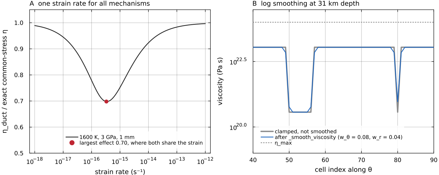
Two of the simplifications measured on the code. Left: the ductile viscosity of composite_rheology (default laws, 1600 K, 3 GPa, 1 mm) divided by the viscosity of an exact parallel combination in which the two mechanisms share one stress and their strain rates add, solved here by bisection. The two agree where one law dominates and differ by up to a factor 0.70 where they share the strain equally. Right: one row at about 30 km depth of a 40 × 120 field in which a band of cells and one isolated cell deform at $3\times {10}^{-13}$ s⁻¹ and yield, before and after _smooth_viscosity. The smoothing widens and rounds the weak zones without leaving the clamp bounds. Script: docs/scripts/fig_rheology_sections.jl.

Configuration summary

field	default	meaning
cfg.useCompositeRheology	false	composite path instead of layered Arrhenius
cfg.eta_min, cfg.eta_max	${10}^{18}$, ${10}^{24}$ Pa s	global clamps
mat.E_act_scale, mat.V_act_scale, mat.T_ref	200 K, 0, 1600 K	simple-path Arrhenius
cfg.useFrankKamenetskii, cfg.fkForm	false, "linearized"	FK law on the simple path
cfg.useDepletionStiffening	false	depletion factor on the simple path
cfg.useSimpleYield	false	yield cap on the simple path (exercised in 2-D only)
mat.harzburgite_eta_factor	3.0	$\xi$ at full residue
cfg.viscosityCombination	"min"	ductile and yield combination
cfg.continentViscosityAveraging	"factor"	continent mixing; "harmonic" averages separately bounded mantle and continent viscosities by the continent fraction
cfg.yieldPressure	"lithostatic"	yield-law pressure; "total" adds the solved Stokes pressure
cfg.smoothViscosity, cfg.smoothStrainRate	true, true	smoothing of the viscosity and of the strain rate the rheology reads
cfg.initialStrainRate	0.0	strain rate of the first viscosity of a fresh run
cfg.yieldMinT	0 K	no yielding below this temperature
cfg.useFullPlasticity	false	strain weakening of the cohesion
cfg.use660kmJump, cfg.eta660kmFactor, cfg.depth660km	false, 30, 660 km	lower-mantle offset (composite path)
cfg.useLayeredActivationEnergy	false	separate lower-mantle $E$, $V$

Tests

• tests/test_composite_rheology.jl: the composite law against the formulas it documents and the physics each creep mechanism must obey.

• tests/test_rheology_switches.jl: the depletion factor $\xi$, the yield temperature gate, the min / harmonic combination, the lower-mantle offset (horizontally averaged ratio equal to eta660kmFactor to a tolerance of 0.05) and depletionStiffensYield, checked on composite_rheology(...; smooth = false).

• tests/test_fk_viscosity.jl, tests/test_arrhenius_viscosity.jl: the helper laws.

• tests/test_depletion_projection.jl: depletion reaches the viscosity and the buoyancy when melting is off.

Key references

• Tian, J., Tackley, P. J. & Lourenço, D. L. (2023). The tectonics and volcanism of Venus: new modes facilitated by realistic crustal rheology and intrusive magmatism. Icarus 399, 115539.

• Austin, N. J. & Evans, B. (2007). Paleowattmeters: a scaling relation for dynamically recrystallized grain size. Geology 35, 343-346.

Further reading

• Schubert, G., Turcotte, D. L. & Olson, P. (2001). Mantle Convection in the Earth and Planets. Cambridge University Press. doi:10.1017/CBO9780511612879

• Turcotte, D. L. & Schubert, G. (2014). Geodynamics, 3rd ed. Cambridge University Press. doi:10.1017/CBO9780511843877

• Karato, S. (2008). Deformation of Earth Materials: An Introduction to the Rheology of Solid Earth. Cambridge University Press. doi:10.1017/CBO9780511804892

• Ranalli, G. (1995). Rheology of the Earth, 2nd ed. Chapman & Hall.

• Gerya, T. (2019). Introduction to Numerical Geodynamic Modelling, 2nd ed. Cambridge University Press. doi:10.1017/9781316534243

• Karato, S. & Wu, P. (1993). Rheology of the upper mantle: a synthesis. Science 260, 771-778. doi:10.1126/science.260.5109.771

• Hirth, G. & Kohlstedt, D. L. (1996). Water in the oceanic upper mantle: implications for rheology, melt extraction and the evolution of the lithosphere. EPSL 144, 93-108. doi:10.1016/0012-821X(96)00154-9

• Hirth, G. & Kohlstedt, D. L. (2003). Rheology of the upper mantle and the mantle wedge: a view from the experimentalists. In Inside the Subduction Factory, AGU Geophysical Monograph 138, 83-105. doi:10.1029/138GM06

• Byerlee, J. (1978). Friction of rocks. Pure and Applied Geophysics 116, 615-626. doi:10.1007/BF00876528

• Kohlstedt, D. L., Evans, B. & Mackwell, S. J. (1995). Strength of the lithosphere: constraints imposed by laboratory experiments. JGR Solid Earth 100, 17587-17602. doi:10.1029/95JB01460

• Mackwell, S. J., Zimmerman, M. E. & Kohlstedt, D. L. (1998). High-temperature deformation of dry diabase with application to tectonics on Venus. JGR Solid Earth 103, 975-984. doi:10.1029/97JB02671

• Christensen, U. (1984). Convection with pressure- and temperature-dependent non-Newtonian rheology. Geophys. J. R. Astron. Soc. 77, 343-384. doi:10.1111/j.1365-246X.1984.tb01939.x

• Solomatov, V. S. (1995). Scaling of temperature- and stress-dependent viscosity convection. Physics of Fluids 7, 266-274. doi:10.1063/1.868624

• Solomatov, V. S. & Moresi, L.-N. (1996). Stagnant lid convection on Venus. JGR Planets 101, 4737-4753. doi:10.1029/95JE03361

• Moresi, L. & Solomatov, V. (1998). Mantle convection with a brittle lithosphere: thoughts on the global tectonic styles of the Earth and Venus. Geophys. J. Int. 133, 669-682. doi:10.1046/j.1365-246X.1998.00521.x

• Tackley, P. J. (2000). Self-consistent generation of tectonic plates in time-dependent, three-dimensional mantle convection simulations, 1. Pseudoplastic yielding. G³ 1, 2000GC000036. doi:10.1029/2000GC000036

• Mitrovica, J. X. & Forte, A. M. (2004). A new inference of mantle viscosity based upon joint inversion of convection and glacial isostatic adjustment data. EPSL 225, 177-189. doi:10.1016/j.epsl.2004.06.005

• Dziewonski, A. M. & Anderson, D. L. (1981). Preliminary reference Earth model. PEPI 25, 297-356. doi:10.1016/0031-9201(81)90046-7