Energy equation

Temperature is advanced in two parts each step: transport by the flow (on markers, or on the grid with an upwind or TVD scheme), then heating and conduction on the grid. This page covers the solver for the second part, diffuse_temperature in solvers/diffuse_temperature.jl. The equation it solves, the conservative radial fluxes and the wall conditions are described in Temperature transport and time stepping.

Schemes

Written for the discrete conduction operator $L$ and heat source $H$,

$$(I-\theta \mathrm{\Delta }tL)T^{n+1}=(I+(1-\theta )\mathrm{\Delta }tL)T^n+\mathrm{\Delta }t\frac{H}{\rho c_p},$$

with

Path	Selected by	$\theta$	Solver
2-D explicit	cfg.useImplicitTemp = false	0 (forward Euler)	none, one stencil update
2-D Crank-Nicolson (default)	cfg.useImplicitTemp = true, cfg.implicitTheta = 0.5	0.5	sparse LU of $I-\theta \mathrm{\Delta }tL$
2-D backward Euler	cfg.implicitTheta = 1.0	1	sparse LU
3-D, time loop	always	0 (forward Euler)	none, one stencil update per patch
3-D, implicit = true keyword	benchmark drivers	1 (backward Euler)	sparse solve per patch

The 2-D matrix $L$ has five entries per row (two radial, two azimuthal neighbours, periodic in $\theta$). It is cached together with the grid, the diffusivity profile and the measure exponent, and rebuilt only if one of them changes. Its LU factor is cached as well and reused while $\mathrm{\Delta }t$ and $\theta$ are unchanged, which happens in fixed-step benchmarks but rarely under CFL control. The wall temperatures enter the right-hand side as sources with the full $\mathrm{\Delta }t$, since they are constant over the step.

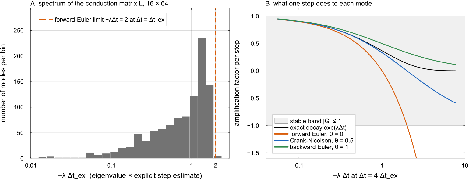
(A) Eigenvalues $\lambda$ of the conduction matrix $L$ that diffuse_temperature builds and caches (_diff_L_cache), on a 16 × 64 spherical annulus, in units of the explicit stability estimate $\mathrm{\Delta }{t}_{\text{ex}}$ of the next figure. All are real and negative; the stiffest reaches $-\lambda \mathrm{\Delta }{t}_{\text{ex}}=1.9$, just inside the forward-Euler limit of 2. (B) Amplification factor per step, $G=[1+(1-\theta )\mathrm{\Delta }t\lambda ]/(1-\theta \mathrm{\Delta }t\lambda )$, of every eigenmode at $\mathrm{\Delta }t=4\mathrm{\Delta }{t}_{\text{ex}}$. Forward Euler leaves the stable band for the stiff modes; Crank-Nicolson stays in it but turns them negative; backward Euler damps them more than the exact decay. Script: docs/scripts/solvers_energy_sections.jl.

Accuracy and stability

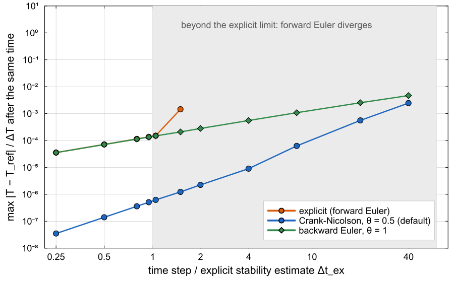
Error of the three 2-D schemes after the same model time, against the time step in units of the explicit stability estimate $\mathrm{\Delta }{t}_{\text{ex}}=1/[\kappa (2/\mathrm{\Delta }{r}^2+2/(r_1\mathrm{\Delta }\theta {)}^2)]$. Spherical annulus $f=0.5$, $32\times 128$ cells, walls at 1300 and 300 K, a 200 K $\cos 4\theta$ anomaly; the reference is Crank-Nicolson with $\mathrm{\Delta }{t}_{\text{ex}}/100$. Forward Euler diverges just above $\mathrm{\Delta }{t}_{\text{ex}}$ (its point at $2\mathrm{\Delta }{t}_{\text{ex}}$ is off the scale). Script: docs/scripts/solvers_energy.jl.

The figure shows the three properties that set the default:

• Order. Crank-Nicolson is second order in time, its error falling by a factor of four when the step halves; forward and backward Euler are first order. At the same step Crank-Nicolson is two to three orders of magnitude more accurate here.

• Stability. Both implicit schemes are unconditionally stable, so in 2-D the time step is set by advection alone (the CFL condition of compute_timestep), and there is no diffusive limit.

• Cost. One sparse solve with a five-point matrix, which is small next to the Stokes solve of the same step.

Backward Euler is more strongly damping: at very large steps Crank-Nicolson can leave a slowly decaying, sign-alternating component in the sharpest modes, which backward Euler removes. Use $\theta =1$ for steady-state searches with large steps and keep $\theta =0.5$ for transient runs.

3-D steps

The explicit 3-D update is stable for $\mathrm{\Delta }t\lesssim \mathrm{\Delta }{x}_{\text{min}}^2/(6\kappa )$. On a stretched grid with thin boundary cells keep cfg.dtMax below that bound.

Coupling the 3-D patches

In 3-D, conduction across the patch boundaries is handled by a short Schwarz iteration of its own. yy_compute_T_wall_bcs samples the peer temperature at each patch's $\theta$-wall faces; both patches are re-diffused with those Dirichlet values (bc_T_jmin, bc_T_jmax keywords), cfg.nTSchwarz times per step (default 3); yy_sync_T_walls! then overwrites each patch's wall-cell row with the peer value at that cell centre. See Yin-Yang Schwarz coupling.

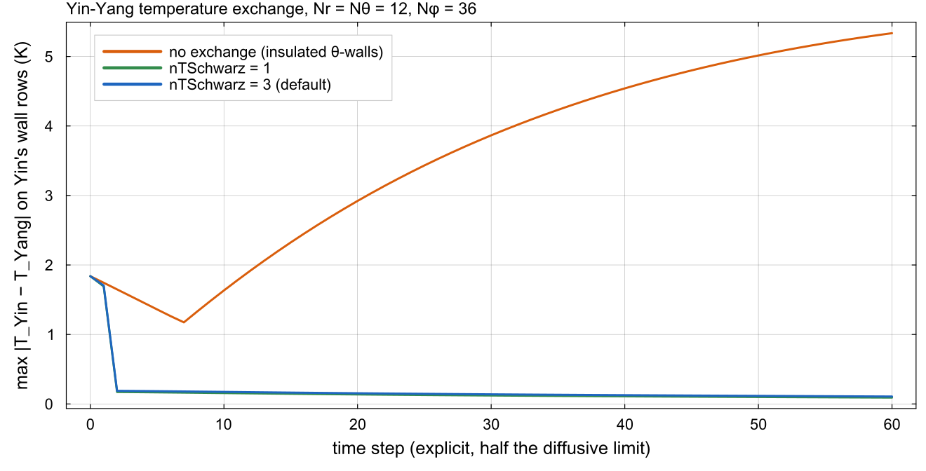
Largest difference between Yin's wall-row temperature and Yang's temperature at the same points, measured before the final yy_sync_T_walls!, on a 3-D shell with $N_r=N_{\theta }=12$, $N_{\phi }=36$. Both patches start from the same field, a conductive profile and a 300 K anomaly centred on Yin's lower $\theta$-wall; the start difference is the bilinear sampling error. Diffused with insulated walls the patches drift apart; with the exchange of the time loop they agree to about 0.1 K after two steps. On this smooth problem one sweep does as well as the default three. Script: docs/scripts/solvers_energy_sections.jl.

Energy conservation

The solver is written so that the discrete energy budget closes: the radial fluxes are differences across cell faces divided by the exact cell measure, and the wall heat flow reported by the diagnostics is the flux the solver itself used. tests/test_nusselt_conduction.jl checks a one-step budget residual of order ${10}^{-15}$ and Nu = 1 on the solver's own conducting state; the logged budget is described in Energy budget.

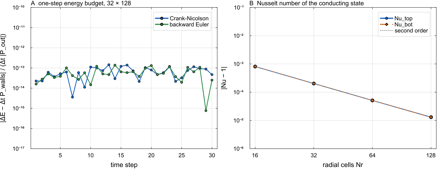
(A) Change of thermal_energy over one call of diffuse_temperature minus $\mathrm{\Delta }t$ times the wall power of boundary_power, weighted with the scheme's own $\theta$, relative to the surface power; 32 × 128 spherical annulus, $\mathrm{\Delta }t=5\mathrm{\Delta }{t}_{\text{ex}}$, 30 consecutive steps from a perturbed conductive field. The residual stays at ${10}^{-13}$, round-off for sums over 4096 cells. (B) Nusselt number from compute_diagnostics on the solver's own conducting steady state, $f=0.55$: top and bottom values coincide and converge to 1 at second order. Script: docs/scripts/solvers_energy_sections.jl.

Where in the code

Topic	File	Function
Entry points (2-D, 3-D)	solvers/diffuse_temperature.jl	diffuse_temperature
Explicit update	solvers/diffuse_temperature.jl	_solve_explicit
θ-scheme, caches	solvers/diffuse_temperature.jl	_solve_crank_nicolson, _diff_L_cache, _diff_lu_cache
3-D wall coupling	utils/yy_interp.jl	yy_compute_T_wall_bcs, yy_sync_T_walls!
Tests	tests/	test_diffusion.jl, test_conduction_conservation.jl, test_nusselt_conduction.jl