Direct solvers

For the 2-D annulus MILEVA factorises the whole Stokes matrix with a sparse direct solver. Two are available on the same assembly:

cfg.solverType	Function	Library
"direct" (default)	solve_stokes_v2 (solvers/solve_stokes_v2.jl)	UMFPACK (Julia's lu), unsymmetric multifrontal LU
"mumps"	solve_stokes_mumps (solvers/solve_stokes_mumps.jl)	MUMPS (Amestoy et al. 2001), multifrontal LU with METIS ordering

A direct solve is exact to round-off at any viscosity contrast: there is no convergence criterion to tune and nothing that degrades as the viscosity field becomes rough. That is why it is the 2-D choice. MUMPS initialises MPI on a single rank by itself, so no MPI launch is needed.

Viscosity contrast. On the 2-D spherical annulus the direct solvers handle viscosity steps up to ${10}^{12}$: MUMPS and UMFPACK give the same velocity to $6\times {10}^{-9}$ or better up to ${10}^9$ on a mid-depth step and to $7\times {10}^{-6}$ at ${10}^{12}$, with the work-dissipation ratio unchanged; a thin stiff lid still solves at ${10}^{18}$. The measurements are on the overview page.

Cost

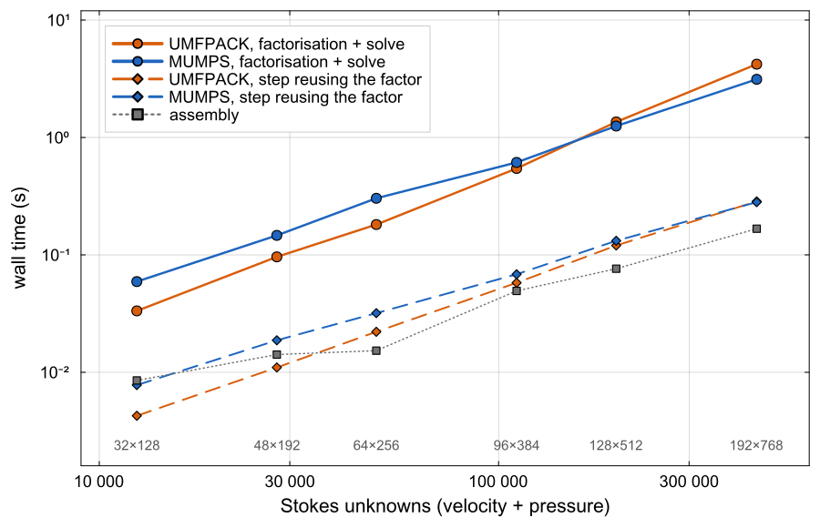
Wall time on the 2-D spherical annulus with a ${10}^6$ viscosity step, from 32 × 128 to 192 × 768 cells. Solid lines: a new factorisation plus solve. Dashed lines: a step that reuses the cached factor, which is only the assembly, the viscosity check and two triangular solves. Dotted: the matrix assembly itself. Measured with two threads on a shared workstation, best of three calls; script docs/scripts/solvers_2d.jl.

Grid ($N_r\times N_t$)	Unknowns	UMFPACK factor + solve	MUMPS factor + solve	Step reusing the factor
32 × 128	12 416	0.03 s	0.06 s	< 0.01 s
64 × 256	49 408	0.18 s	0.30 s	0.02 to 0.03 s
96 × 384	110 976	0.54 s	0.61 s	0.06 to 0.07 s
128 × 512	197 120	1.36 s	1.25 s	0.12 to 0.13 s
192 × 768	443 136	4.2 s	3.1 s	0.28 s

On the point-pinned assembly the two libraries cost about the same up to $2\times {10}^5$ unknowns, and MUMPS pulls ahead above that. Their cost grows as $N^{1.1}$ to $N^{1.4}$ over this range, close to the $N^{1.5}$ expected for nested-dissection orderings on a 2-D mesh. The viscosity contrast does not change either cost measurably. MUMPS is the better choice for large 2-D grids and for runs that use the stale-factor preconditioner below, which only MUMPS offers; at production sizes up to $N_r\approx 128$ either is fine.

Pressure pin

Pressure enters the incompressible Stokes equations only through its gradient, so it is fixed up to a constant. All 2-D solvers remove that null space by pinning the pressure at a single cell (point_pin = true in assemble_stokes): the continuity row of that cell is replaced by an identity row. The alternative, a dense "mean pressure = 0" row, couples every pressure unknown, which fills the factor and is badly handled by MUMPS at large viscosity contrast. With the point pin MUMPS and UMFPACK agree to $2\times {10}^{-13}$ on a ${10}^6$-contrast annulus.

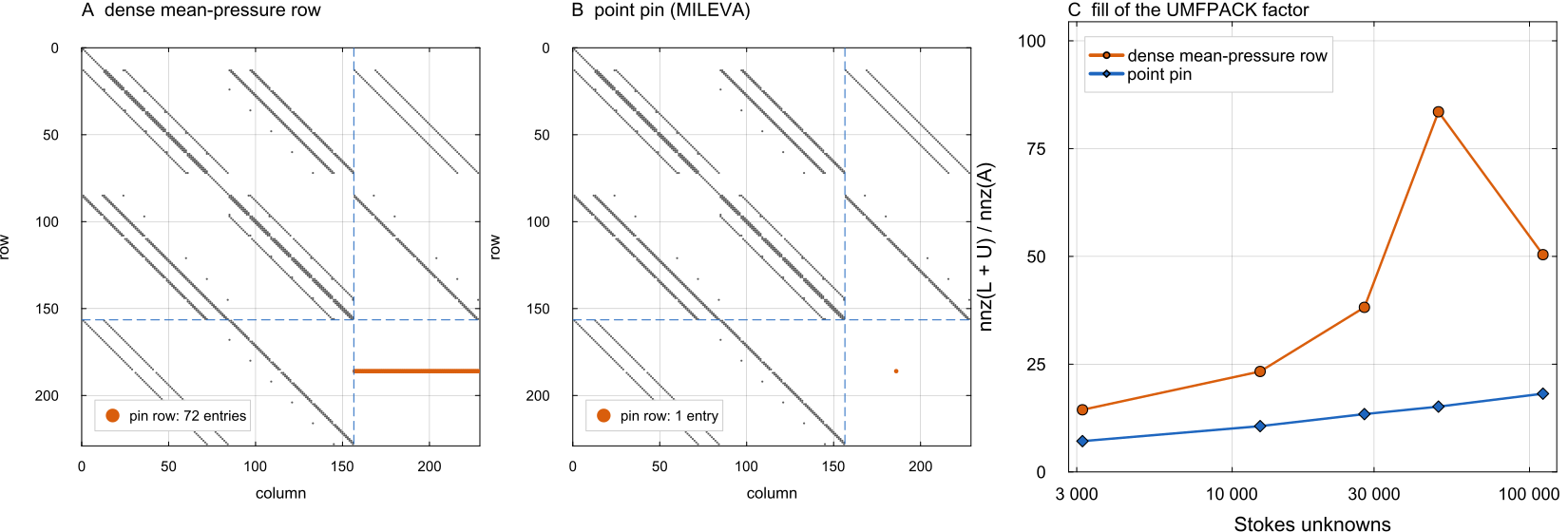
(A, B) Nonzero pattern of the 2-D Stokes matrix from assemble_stokes on a 6 × 12 annulus; dashed lines separate the velocity unknowns from the pressure unknowns, and the pin row is drawn in orange. The dense row couples all 72 pressure unknowns; the point pin is a single diagonal entry. (C) Fill of the UMFPACK factor, entries of $L+U$ over entries of the matrix, from 16 × 64 to 96 × 384 cells with a ${10}^6$ viscosity step: with the dense row the factor is two to five times larger. Script: docs/scripts/solvers_direct_sections.jl.

No pressure penalty is added to the continuity rows (cfg.pPen = 0): the staggered grid is stable without one, and the direct solvers return a discretely divergence-free velocity to round-off, the pinned cell included.

Reusing the factorisation

Both direct solvers keep their factorisation, together with the viscosity field it was built from, in a module-level cache. On the next call the largest relative change in viscosity,

$$\underset{ij}{max}\frac{|{\eta }_{ij}-{\eta }_{ij}^{\text{cached}}|}{|{\eta }_{ij}^{\text{cached}}|+1},$$

is compared with the tolerance (cfg.luCacheTol for MUMPS, default ${10}^{-4}$). Below it the old factor is reused and only the triangular solves run, which is about ten times cheaper (dashed lines above). Isoviscous benchmarks take this path every step. Runs with temperature- and stress-dependent viscosity change the field by more than that almost every step, so a full refactorisation is the norm there.

Stale-factor preconditioning (MUMPS). With cfg.luReuseMaxIter > 0 a factor that is out of date is not thrown away. It becomes a right preconditioner for a short GMRES on the current operator, warm-started from the previous solution, and the solver refactorises only when GMRES needs more than luReuseMaxIter iterations to reach cfg.luReuseTol (default ${10}^{-11}$). The answer is still exact to that tolerance. The time loop reports how many solves took this path at the end of the run (lu_reuse_stats).

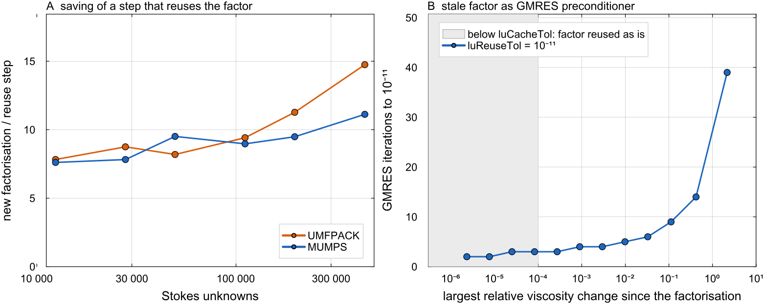
(A) Time of a new factorisation and solve divided by the time of a step that reuses the cached factor, from the measurements of the Cost figure. (B) GMRES iterations (_gmres_right_precond_3d, the routine of the stale-factor path) to a relative residual of ${10}^{-11}$ when the exact factor of one viscosity field preconditions the operator of a perturbed field, against the largest relative viscosity change of the formula above; 64 × 256 cells, a smooth field spanning three orders of magnitude. Below luCacheTol the factor is reused without iteration (shaded). Script: docs/scripts/solvers_direct_sections.jl.

BiCGSTAB ("amg")

solve_stokes_amg runs unpreconditioned BiCGSTAB($\ell$ = 2) from IterativeSolvers.jl. No algebraic multigrid is built: the velocity block is non-symmetric because of the curvature and cross-coupling terms of the full stress, and smoothed-aggregation AMG built on its symmetric part made the iteration worse. If BiCGSTAB does not reach $max(\mathtt{\text{krylovTol}},{10}^{-10})$ the routine falls back to MUMPS. On the test problem of the figures above it falls back every time, so it costs a direct solve plus the failed iteration.

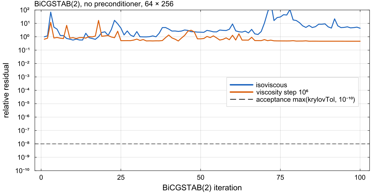
Recurrence residual of IterativeSolvers.bicgstabl ($\ell$ = 2) with the settings of solve_stokes_amg on the 64 × 256 annulus of the Cost figure, up to the cap of $2\mathtt{\text{krylovMaxIter}}$ matrix-vector products. Neither case approaches the acceptance level (dashed), so both end in the MUMPS fallback. The shadow residual is random; the seed is fixed for the figure. Script: docs/scripts/solvers_direct_sections.jl.

Where in the code

Topic	File	Function
UMFPACK path and cache	solvers/solve_stokes_v2.jl	solve_stokes_v2, _lu_cache
MUMPS path, cache, stale-factor GMRES	solvers/solve_stokes_mumps.jl	solve_stokes_mumps, _mumps_cache, lu_reuse_stats
BiCGSTAB with fallback	solvers/solve_stokes_amg.jl	solve_stokes_amg
Assembly and pin	solvers/stokes_assembly.jl	assemble_stokes(...; point_pin = true)
Tests	tests/	test_stokes.jl

Reference. Amestoy, P. R., Duff, I. S., L'Excellent, J.-Y. and Koster, J. (2001), A fully asynchronous multifrontal solver using distributed dynamic scheduling, SIAM J. Matrix Anal. Appl. 23, 15-41. Davis, T. A. (2004), Algorithm 832: UMFPACK V4.3, an unsymmetric-pattern multifrontal method, ACM Trans. Math. Softw. 30, 196-199.