Free surface and isostasy

MILEVA's top boundary is the fixed sphere $r=R_{\text{out}}$ with free slip and $V_r=0$ (see Governing equations). The mesh never moves. Three options approximate a deformable surface on top of that; they differ in whether they change the flow at all.

option	switch	changes the Stokes solution	output
sticky air	cfg.useStickyAir	yes: a weak, buoyancy-free layer inside the domain	the flow itself
kinematic surface tracker	cfg.useFreeSurface	no	internal deflection field
relaxed isostatic topography	cfg.useIsostasy	no	internal deflection field

All three default to false.

Physical background

Free surface and free slip

The surface of a planet is a free surface. Nothing above it (vacuum, an atmosphere or an ocean) can exert a shear stress worth mentioning on the rock, and the boundary moves with the material that forms it. Mathematically that is two conditions. The traction on the surface vanishes, $\mathit{\sigma }\cdot \hat{\mathbf{n}}=0$ (apart from the small pressure of whatever lies on top), and the surface is kinematic, meaning that a point on it stays on it, so its height changes only where the flow carries material up, down or sideways across a slope.

Most global convection models replace this with free slip on a fixed sphere: zero shear traction but zero normal velocity. The reason is scale. Surface topography on Earth and Venus is a few kilometres, while the mantle is close to 3000 km deep, so the shape of the domain hardly changes. The flow still pushes on the rigid lid of the domain, and the normal stress it exerts there is the stress a real surface would have to balance with its own weight. Converting one into the other gives the classic estimate of dynamic topography (Hager et al. 1985; Zhong, Gurnis & Moresi 1996),

$$h_{\text{dyn}}=-\frac{\delta {\sigma }_{rr}}{\mathrm{\Delta }\rho g},$$

where $\delta {\sigma }_{rr}$ is the lateral deviation of the radial normal stress on the boundary (tension positive), $\mathrm{\Delta }\rho$ the density contrast across the surface and $g$ gravity. Above an upwelling the mantle presses up on the boundary (compressive $\delta {\sigma }_{rr}$) and the surface rises; above a downwelling it pulls down and the surface sinks. The options on this page do not use the normal stress; they are three other ways of letting a surface respond, described below.

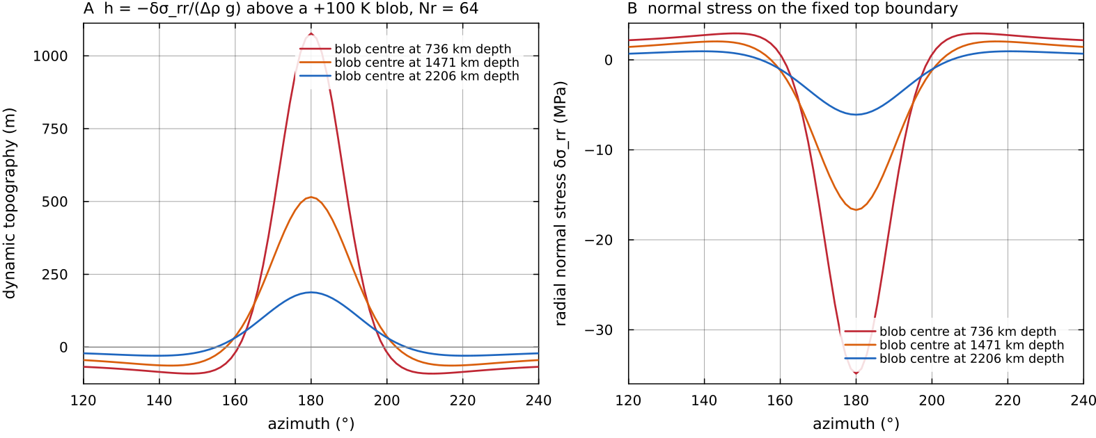
The classic estimate evaluated on a free-slip Stokes solution, as a post-processing illustration (no MILEVA option computes it): assemble_stokes on a Venus-sized spherical annulus, 64 × 256 cells, Boussinesq, $\eta ={10}^{21}$ Pa s, with a +100 K blob centred at three depths. B: the lateral deviation of ${\sigma }_{rr}=-P+2\eta \partial V_r/\partial r$ in the top cell, compressive above the blob. A: $h=-\delta {\sigma }_{rr}/({\rho }_{0}g)$, a swell of 1080, 520 and 190 m that weakens and widens as the blob deepens. Script: docs/scripts/fig_free_surface_sections.jl.

Isostatic and dynamic topography

Topography is supported in two broad ways. Isostatic topography floats. A column of lithosphere that is lighter than its neighbours stands higher, one that is heavier stands lower, and below some compensation depth the pressure is the same everywhere. Airy compensation achieves this with thickness changes of a light crust (mountains with roots), Pratt compensation with lateral density changes at fixed thickness, and flexural compensation spreads the load over a region through the bending strength of an elastic plate (Watts 2023). Dynamic topography is held up or pulled down by the stresses of the flow beneath the lithosphere and disappears when that flow stops.

Thermal isostasy is the example that matters most for a convecting planet. A conductive lid is colder, and therefore denser, than the mantle beneath it. Where the lid is thicker the column carries more mass and sinks. This is why the ocean floor deepens as the plate ages and thickens, roughly with the square root of age (Parsons & Sclater 1977). For a lid with a linear temperature profile from $T_s$ to $T_m$, the mean temperature deficit is $(T_m-T_s)/2$, so thickening the lid by $\mathrm{\Delta }L$ adds a mass excess ${\rho }_0\alpha (T_m-T_s)\mathrm{\Delta }L/2$ per unit area. Balancing that against mantle of density ${\rho }_0$ displaced at the surface gives a deflection

$$\mathrm{\Delta }h\approx -\frac{1}{2}\alpha (T_m-T_s)\mathrm{\Delta }L.$$

With $\alpha =3\times {10}^{-5}$ K${}^{-1}$, $T_m-T_s=1300$ K and $\mathrm{\Delta }L=40$ km (the lid of the figures below) this is about $-780$ m. The isostasy figure gives $-747$ m at the thickest point; the difference is mainly that isostasy measures density against the mean of each radial row, and that mean already contains part of the thick lid.

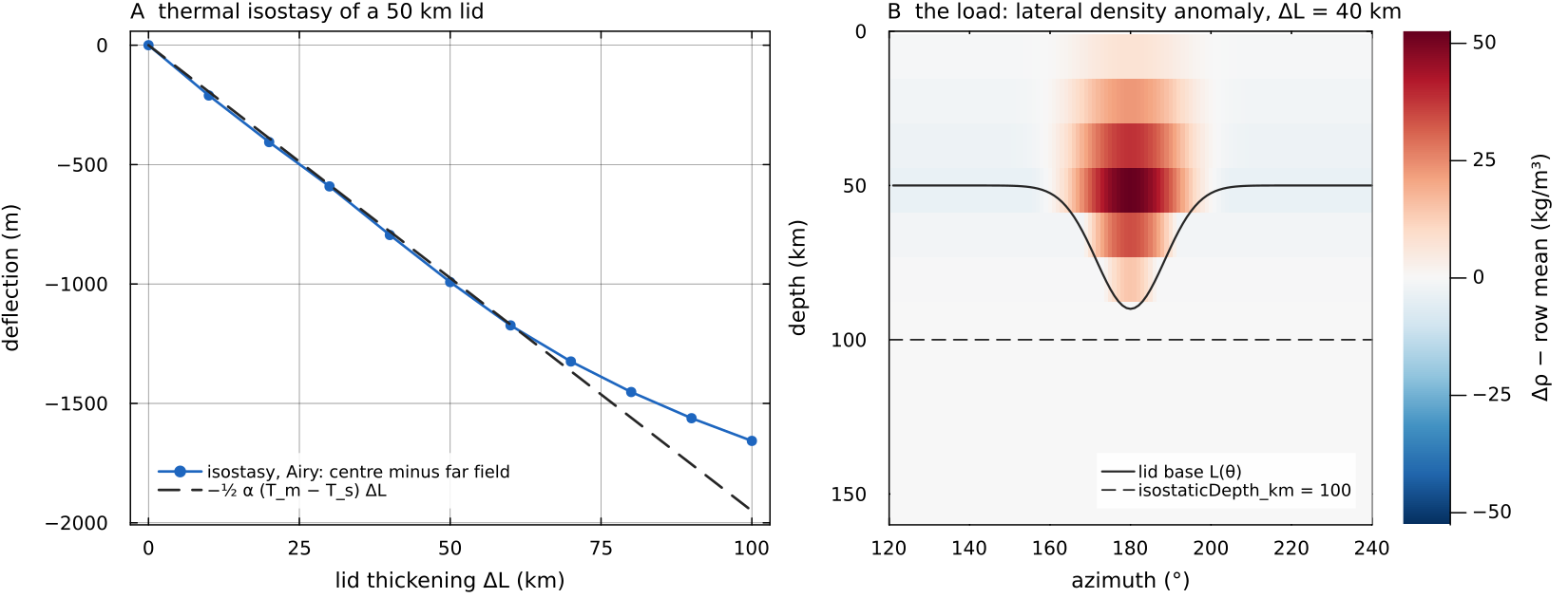
A: the Airy equilibrium of isostasy at the lid centre, relative to the far field, for a 50 km conductive lid thickened by 0 to 100 km (200 × 360 annulus), against $-\frac{1}{2}\alpha (T_m-T_s)\mathrm{\Delta }L$. The two agree while the root stays inside the 100 km compensation layer (795 m against 780 m at 40 km) and part as the root grows past it, since isostasy counts only the top 100 km. B: the load for $\mathrm{\Delta }L$ = 40 km, the density anomaly against each row's mean, with the lid base and the compensation depth. Script: docs/scripts/fig_free_surface_sections.jl.

How fast topography relaxes

A surface that is out of equilibrium relaxes by viscous flow of the mantle below it. For a Newtonian half-space of viscosity $\eta$ and a sinusoidal topography of wavelength $\lambda$, the amplitude decays exponentially with time constant

$$\tau =\frac{4\pi \eta }{\rho g\lambda }$$

(Haskell 1935; Turcotte & Schubert 2014). With $\eta ={10}^{21}$ Pa s, $\rho =3300$ kg/m³ and $g=9.81$ m/s², $\tau$ is about 12 000 yr at $\lambda$ = 1000 km and about 4 100 yr at $\lambda$ = 3000 km. That is the timescale of postglacial rebound, and three to four orders of magnitude shorter than the tens to hundreds of million years over which mantle convection reorganises. At long wavelengths, therefore, the surface is effectively always in equilibrium with the stresses below it, which is what justifies free slip plus a computed topography. The argument weakens at short wavelengths and beneath a very stiff lid, where topography grows on timescales comparable to convection itself and depends on its own history (Zhong, Gurnis & Moresi 1996).

The same short relaxation time makes a truly free surface awkward to compute. If a time step is longer than the relaxation time of the shortest resolved wavelength, an explicit update overshoots, and the surface swings up and down with growing amplitude from step to step. Kaus, Mühlhaus & May (2010) named this the "drunken sailor" instability and proposed the stabilisation that free_surface borrows in a simplified form.

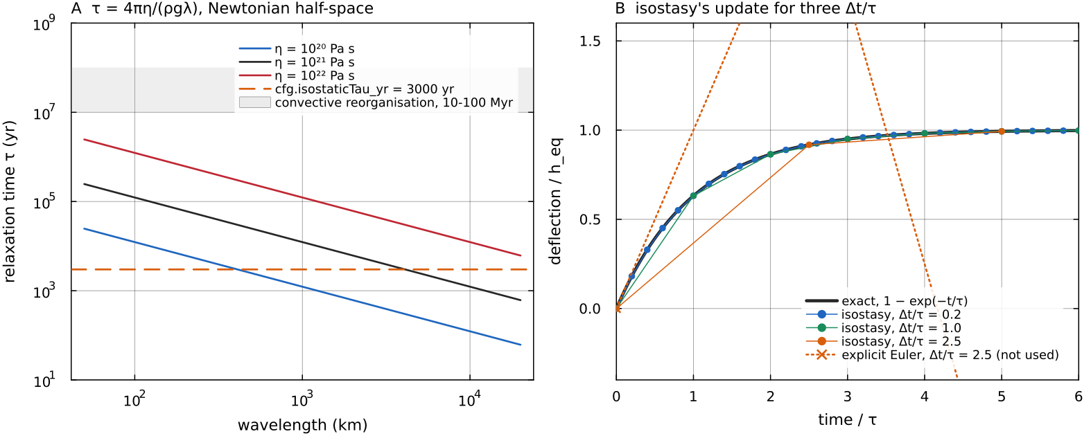
A: the half-space relaxation time $4\pi \eta /(\rho g\lambda )$ for three viscosities, against the default isostaticTau_yr and the time over which convection reorganises. B: the deflection at the centre of the thickened lid stepped by isostasy with $\mathrm{\Delta }t/\tau$ = 0.2, 1 and 2.5; every step lands on the exact curve $1-e^{-t/\tau }$, whatever its length. An explicit Euler step of the same law (dotted, not used by the code) overshoots and oscillates with growing amplitude at $\mathrm{\Delta }t/\tau$ = 2.5. Script: docs/scripts/fig_free_surface_sections.jl.

Flexure

An elastic plate of thickness $T_e$, Young's modulus $E$ and Poisson's ratio $\nu$ resists bending with flexural rigidity $D=E{T}_e^3/[12(1-{\nu }^2)]$. Loaded at wavenumber $k$ (wavelength $2\pi /k$) and supported from below by a fluid of density $\rho$, it deflects by the Airy amount multiplied by the response function

$$\mathrm{\Phi }(k)=\frac{\rho g}{D{k}^4+\rho g}$$

(Watts 2023). Long loads ($D{k}^4\ll \rho g$) are compensated locally, as in Airy isostasy; short loads ($D{k}^4\gg \rho g$) are carried by the plate's strength and barely deflect it. The length that separates the two is the flexural parameter ${\alpha }_f=[4D/(\rho g){]}^{1/4}$. For the MILEVA defaults ($T_e$ = 30 km, $E$ = 70 GPa, $\nu$ = 0.25, ${\rho }_0$ = 3300 kg/m³, $g$ = 9.81 m/s²), $D=1.68\times {10}^{23}$ N m, ${\alpha }_f\approx 67$ km, and the response falls to one half at a wavelength of about 300 km, that is azimuthal wavenumber about 133 on a planet of radius 6371 km.

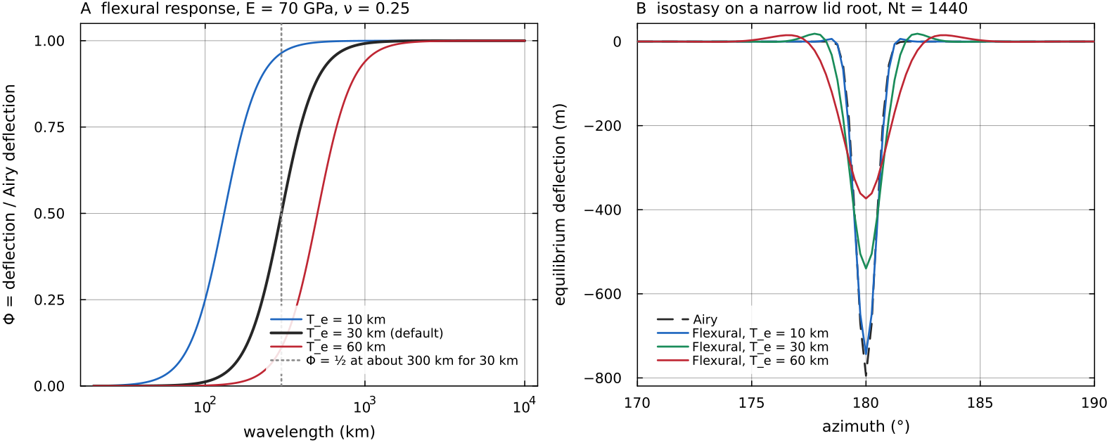
A: the response $\mathrm{\Phi }(k)$ for elastic thicknesses of 10, 30 (default) and 60 km. B: isostasy in Airy and in Flexural mode on a lid root about 70 km wide, on a 200 × 1440 annulus. The flexural branch calls a Fourier transform; FFTW is not a dependency of the repository, so the script supplies a plain discrete transform under the name the code looks for, and the spectral solve itself is MILEVA's. A 10 km plate barely changes the Airy answer, a 60 km plate halves the depression, spreads it and raises a small flexural bulge on each side. Script: docs/scripts/fig_free_surface_sections.jl.

Scales and typical values

Three ratios decide which approximation is adequate:

$$\mathrm{\Delta }t/\tau$$

, the time step against the relaxation time. When it is large the surface reaches equilibrium within each step; when it is of order one or larger for a resolved wavelength, an explicit free surface needs stabilisation.

• $$h/\lambda$$

  , topography against its wavelength. Small values justify a fixed mesh with the deflection treated as a small perturbation (Zhong, Gurnis & Moresi 1996 find their fixed-grid free surface accurate in this limit).

• $$({\eta }_{\text{st}}/{\eta }_{\text{ch}})(L/h_{\text{st}}{)}^3$$

  , the sticky-air criterion of Crameri et al. (2012), discussed under Sticky air.

quantity	value	source
observed dynamic topography, Earth, ~10³ km wavelength	typical peak amplitude ±1 km	Hoggard, White & Al-Attar 2016
observed dynamic topography, Earth, ~10⁴ km wavelength	peak amplitude about ±500 m	Hoggard, White & Al-Attar 2016
Venus hypsometry	unimodal; more than 80 % of the surface lies within 1 km of the 6051.84 km mean radius	Ford & Pettengill 1992
Venus support of topography	about 10 % of the surface (highland plateaus, tesserae) consistent with crustal-thickness compensation; the remaining 90 % (rises, plains, lowlands) dominated by convective tractions	Simons, Solomon & Hager 1997
Venus elastic thickness	below 20 km at highland plateaus and tesserae when their relief formed; below 30 km at highland rises	Simons, Solomon & Hager 1997
relaxation time, $\eta ={10}^{21}$ Pa s, $\lambda$ = 1000 to 3000 km	about 12 000 to 4 100 yr	computed from Haskell (1935) above

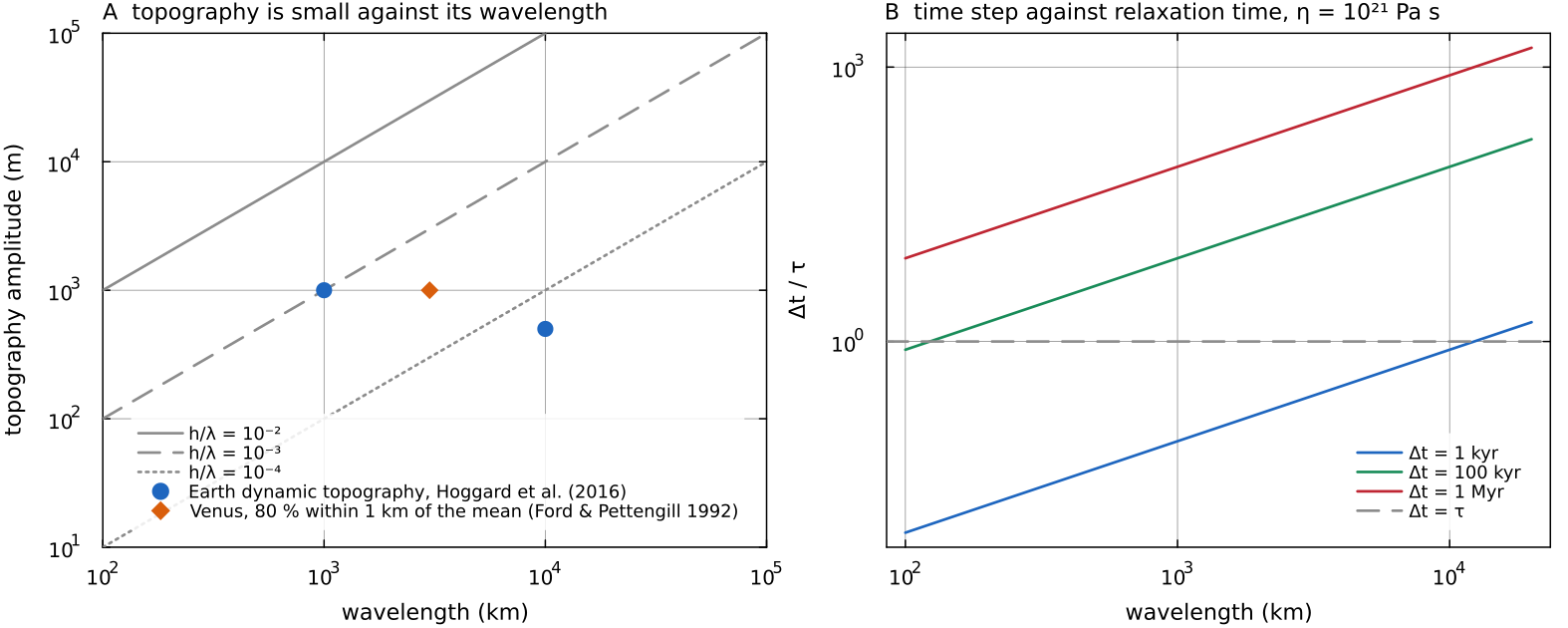
A: the observed amplitudes of the table against their wavelengths, with lines of constant $h/\lambda$. All lie at or below ${10}^{-3}$, the small-topography limit. B: $\mathrm{\Delta }t/\tau$ for time steps of 1 kyr, 100 kyr and 1 Myr at ${10}^{21}$ Pa s. At the time steps of a mantle convection run, 100 kyr and longer, the surface is relaxed within one step at every wavelength longer than about 100 km. Script: docs/scripts/fig_free_surface_sections.jl.

Sticky air

apply_sticky_air! (utils/sticky_air.jl) overrides every cell whose centre lies within cfg.airThickness (80 km) of $R_{\text{out}}$: its viscosity becomes cfg.airViscosity (${10}^{18}$ Pa s) and its buoyancy becomes cfg.airDensity (1.0, written into the force-density field, so about 1 N m${}^{-3}$, effectively zero). The mantle below then sees a nearly stress-free upper boundary at the base of the air layer, which can deflect with the flow (Schmeling et al. 2008; Crameri et al. 2012). It is applied after the buoyancy and viscosity are built and before the Stokes solve, in 2-D and 3-D.

Notes on the implementation:

• the air layer is a fixed set of whole radial rows, chosen by cell centre; it is not a material, so mantle carried into it takes on air properties and air does not follow the interface;

• the layer must be thicker than the top cell or nothing is overridden (the code warns);

• the quality of the approximation depends on the air-to-mantle viscosity ratio and the layer thickness (Crameri et al. 2012); the default is ${10}^{18}$ Pa s; test it for the problem at hand.

Why the method works, and when it does not, follows from the relaxation argument above. The air layer must be weak enough that the shear and normal stresses it transmits to the mantle are negligible over the time the surface takes to adjust, and thick enough that it does not itself act as a stiff lid on the flow. Crameri et al. (2012) compared sticky-air topography with true free surfaces in several codes and found the approximation good as long as

$$C_{\text{st}}=\frac{{\eta }_{\text{st}}}{{\eta }_{\text{ch}}}{\left(\frac{L}{h_{\text{st}}}\right)}^3$$

is sufficiently small, where ${\eta }_{\text{st}}$ and $h_{\text{st}}$ are the viscosity and thickness of the air layer and ${\eta }_{\text{ch}}$ and $L$ a characteristic viscosity and length of the model. The cube makes the thickness the stronger lever. For the defaults (${\eta }_{\text{st}}={10}^{18}$ Pa s, $h_{\text{st}}$ = 80 km) and ${\eta }_{\text{ch}}={10}^{21}$ Pa s, $C_{\text{st}}$ is about 0.6 for $L$ = 660 km and about 50 for $L$ = 2890 km, the depth of the default shell. Which length is the relevant one depends on the wavelength of the topography the problem cares about.

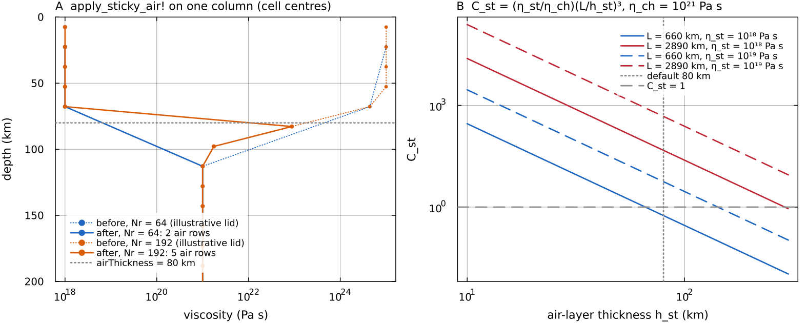
A: apply_sticky_air! on one column of an illustrative lid, at 64 and 192 radial cells (default Earth-sized shell). Whole rows whose centre lies within 80 km of the surface are set to ${10}^{18}$ Pa s: two rows (down to 90 km) on the 45 km cells of Nr = 64, five rows (down to 75 km) on the 15 km cells of Nr = 192. B: the criterion $C_{\text{st}}$ against the air-layer thickness for two lengths and two air viscosities, with the default 80 km. Script: docs/scripts/fig_free_surface_sections.jl.

Kinematic surface tracker

The two deflection options work as a short chain inside each time step. First the tracker reads the flow at the top of the mantle and carries the surface shape with it: it measures how steep the surface is, works out how fast the sideways flow moves that shape (the top face has no vertical velocity, so the flow alone cannot raise or lower the surface), takes a damped step forward in time and filters the result to damp grid-scale wiggles at a rate set by how fast the surface flow crosses a cell. Then the isostasy routine looks down the top 100 km of each column, adds up how much heavier or lighter it is than the average column, turns that excess mass into the height at which the column would float, and lets the surface relax part of the way toward that height. The figure follows one step through both routines for two columns.

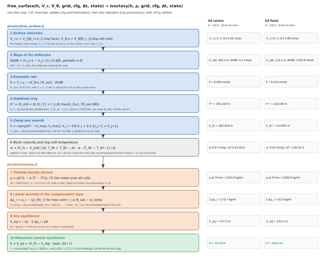
One 1 kyr step of free_surface followed by isostasy in Airy mode, on a 200 x 360 annulus with a conductive lid thickened from 50 to 90 km (the field of the isostasy figure below) and a prescribed surface velocity $V_{\theta }$ = 5 cm/yr $\cos (\theta -\pi )$. Left values: the lid centre at $\theta$ = 180°, where the surface is flat and the deflection moves from −363.4 m toward the Airy equilibrium −747.3 m, ending at −471.8 m. Right values: the flank at $\theta$ = 168°, slope −1321 m/rad, moving from −118.2 m toward −242.2 m and ending at −154.0 m. Both switches are off by default and are turned on for the example; the script checks every stage against the two functions. Script: docs/scripts/fig_free_surface_pipeline.jl.

free_surface (physics/free_surface.jl) advances a surface deflection $h(\theta )$ (2-D) or $h(\theta ,\varphi )$ (3-D) after each Stokes solve with the kinematic condition

$$\frac{\partial h}{\partial t}=V_r-\frac{V_{\theta }}{R_{\text{out}}}\frac{\partial h}{\partial \theta }(\text{3-D: }-\frac{V_{\varphi }}{R_{\text{out}}\sin \theta }\frac{\partial h}{\partial \varphi }),$$

where

symbol	meaning	in the code
$h$	surface deflection above (positive) or below $R_{\text{out}}$, m	h_surf in main_SphCon.jl
$V_r$	radial velocity on the top face	Vr[end, :] (2-D), Vr[Nr+1, :, :] (3-D)
$V_{\theta }$, $V_{\varphi }$	tangential velocities in the top cell row	Vt[end, :]; 3-D: Vth averaged to the cell centre, Vph at a $\varphi$ face
$R_{\text{out}}$	outer radius of the fixed mesh	grid.R_out
$\partial h/\partial \theta$, $\partial h/\partial \varphi$	surface slopes, centred differences, periodic in the annulus and in $\varphi$	one-sided at the 3-D $\theta$ walls

The equation says that the surface height at a fixed angle changes for two reasons: material crossing the surface vertically ($V_r$), and an existing slope being carried sideways by the tangential flow (the advection term). Because the Stokes solve keeps $V_r=0$ on the top face, only the second term is non-zero in MILEVA, so the tracker moves an existing deflection along the surface but cannot create one. On its first call the tracker starts from the deflection it is given.

The tracker uses $V_r$ on the top face and $V_{\theta }$ in the top cell row. The update is divided by $1+f_s\mathrm{\Delta }tmax|V_{\theta }|/(R_{\text{out}}\mathrm{\Delta }\theta )$ (a one-pass linearised form of the Kaus et al. 2010 stabilisation, $f_s$ = cfg.freeSurfaceStabilization, 0.5), clamped to $\pm$cfg.freeSurfaceMaxDrop (50 km) and filtered with a three-point (2-D) or five-point (3-D) stencil. The filter is rate based: its weight is chosen so that the grid-scale (two-cell) mode is multiplied by $e^{-\mathrm{\Delta }t/{\tau }_f}$ per step, with ${\tau }_f=R_{\text{out}}\mathrm{\Delta }\theta /max|V_{\theta }|$ (3-D: the smaller angular spacing and the larger tangential speed) the time the surface flow takes to cross one cell. A given model time therefore damps that mode by the same amount whatever the number of steps, for $\mathrm{\Delta }t\ll {\tau }_f$ the filter is a diffusion of $h$ with diffusivity $(R_{\text{out}}\mathrm{\Delta }\theta {)}^2/(4{\tau }_f)$ (half that in 3-D), and a surface with no tangential flow is not filtered at all. The deflection rate $w=\mathrm{\Delta }h/\mathrm{\Delta }t$ is then used to correct the top-cell temperature, $T_{N_r}\leftarrow T_{N_r}-\mathrm{\Delta }tw\partial T/\partial r$.

Two details of this chain are worth stating precisely. First, the stabilisation in Kaus, Mühlhaus & May (2010) is a correction term added to the momentum equation, which accounts for the density that moves across the surface during a time step. MILEVA applies its version to the tracker update only. Since the denominator is larger than 1 whenever the surface moves sideways, it damps the deflection by the same factor everywhere in that step, on top of the advection. Second, $w$ is the rate produced by free_surface alone, stored as state_fs.w_mesh; the later isostatic adjustment changes $h$ but not $w$, so the top-cell temperature correction sees only the tracker's change. The temperature gradient in that correction is the one-sided difference between the top two cells, divided by the distance between their centres, grid.r[Nr] - grid.r[Nr-1] (surface_motion_temperature_correction!).

Deformable surface

The Stokes solve keeps $V_r=0$ on the top face and the mesh fixed, so the tracker advects and filters a deflection supplied by useIsostasy. For a mechanically deformable surface use sticky air.

Isostatic topography

isostasy (physics/isostasy.jl) relaxes a surface deflection toward isostatic equilibrium with the density of the top cfg.isostaticDepth_km (100 km). The driver passes a thermal density $\rho ={\rho }_0[1-\alpha (T-\bar{T})]$ with $\bar{T}$ the mean over the whole domain, and the routine works with the lateral anomaly $\mathrm{\Delta }\rho =\rho -⟨\rho {⟩}_r$ at each radius.

Airy (cfg.isostaticMode = "Airy", 2-D and 3-D): local column compensation,

$$h_{\text{eq}}=-\frac{1}{{\rho }_0}\sum _{z_i<d_{\text{comp}}}\mathrm{\Delta }{\rho }_i\mathrm{\Delta }{r}_i.$$

This is the statement that every column carries the same mass above the compensation depth. A column with an excess mass $\sum \mathrm{\Delta }{\rho }_i\mathrm{\Delta }{r}_i$ per unit area sinks until the mantle it no longer occupies at the top, ${\rho }_0{h}_{\text{eq}}$ per unit area, cancels the excess; the material above the surface is taken to have zero density. Here $\mathrm{\Delta }{r}_i$ is the radial width of cell $i$ (grid.drVec[i]), $z_i$ the depth of cell centre $i$, $d_{\text{comp}}$ = cfg.isostaticDepth_km, $\mathrm{\Delta }{\rho }_i$ the lateral density anomaly of cell $i$ in that column and ${\rho }_0$ = cfg.rho0. A dense (cold, thick) column gives a negative $h_{\text{eq}}$, a depression. Since the anomaly is measured against the row mean, $h_{\text{eq}}$ describes the shape of the surface relative to its mean level, not the absolute radius.

Flexural ("Flexural", 2-D only): a thin elastic plate solved spectrally in the azimuthal wavenumber $k$,

$$[D(\frac{k}{R_{\text{out}}}{)}^4+{\rho }_{0}g]{\hat{H}}_k=-{\hat{Q}}_k,Q=g\sum _{z_i<d_{\text{comp}}}\mathrm{\Delta }{\rho }_i\mathrm{\Delta }{r}_i,$$

with rigidity $D$ = cfg.flexuralRigidity, or, when that is 0, $D=E{T}_e^3/[12(1-{\nu }^2)]$ from cfg.elasticThickness_km (30 km), $E=70$ GPa and $\nu =0.25$. The mean deflection is set to zero. The spectral solve needs FFTW loaded in the session; otherwise it falls back to Airy with a warning. The 3-D dispatch accepts only Airy.

In this equation ${\hat{Q}}_k$ and ${\hat{H}}_k$ are the discrete Fourier coefficients of the load $Q$ (in Pa) and of the equilibrium deflection around the annulus, $k$ is the integer azimuthal wavenumber, so $k/R_{\text{out}}$ is the physical wavenumber along the surface, and ${\rho }_{0}g$ is the restoring pressure per metre of deflection. Dividing by ${\rho }_{0}g$ shows that each harmonic is the Airy deflection times the response function $\mathrm{\Phi }$ of the Flexure background, so the same load is compensated locally at long wavelength and carried by the plate at short wavelength.

The topography relaxes toward equilibrium with time constant $\tau$ = cfg.isostaticTau_yr (3000 yr):

$$h(t+\mathrm{\Delta }t)=h_{\text{eq}}+[h(t)-h_{\text{eq}}]e^{-\mathrm{\Delta }t/\tau }.$$

This is the exact solution over one step of the first-order relaxation law $\mathrm{d}h/\mathrm{d}t=-(h-h_{\text{eq}})/\tau$ with $h_{\text{eq}}$ held fixed, so it is stable for any time step. The ratio $\mathrm{\Delta }t/\tau$ decides what the update does. For $\mathrm{\Delta }t\gg \tau$ the factor $e^{-\mathrm{\Delta }t/\tau }$ vanishes and $h$ is simply $h_{\text{eq}}$; for $\mathrm{\Delta }t$ = 1 kyr and the default $\tau$ = 3000 yr, as in the pipeline figure, 72 % of the remaining gap survives each step. A single $\tau$ stands in for the wavelength-dependent relaxation time of the background.

The load is thermal. The column sum weights each row by its own cell width, so the deflection is the same column integral on uniform and stretched radial grids. The relaxation time is converted to seconds with cfg.SEC_PER_MYR in both 2-D and 3-D. The deflection is a diagnostic of the loop and is not written to the output files.

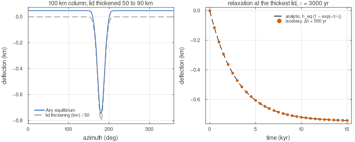
isostasy in Airy mode on a thermal density field whose conductive lid thickens from 50 to 90 km over about 40 degrees of azimuth. Left: the equilibrium deflection, a depression over the thick, dense lid that follows its shape. Right: the deflection at the thickest lid, stepped with 500 yr steps, against the exact exponential approach with the default $\tau$ = 3000 yr.

Assumptions and simplifications

• The mesh and the mechanical boundary stay fixed. The Stokes solve always sees $V_r=0$ and free slip on $r=R_{\text{out}}$. Of the three options only sticky air changes the flow; the tracker and isostasy compute a deflection that is not fed back into the momentum equation. This is the small-topography limit of the background section, reasonable when $h\ll \lambda$ and the surface relaxes much faster than the flow evolves.

• The deflection reaches the temperature field only through the top cell. The tracker's rate $w$ shifts the top-cell temperature as if the surface had moved through the thermal gradient; nothing else in the model sees $h$.

• Isostatic loads are thermal. The density passed to isostasy is ${\rho }_0[1-\alpha (T-\bar{T})]$; composition, melt and phase changes do not enter it, and the material above the surface has zero density.

• One compensation depth and one relaxation time. Both are constants (cfg.isostaticDepth_km, cfg.isostaticTau_yr), where in nature the relaxation time depends on wavelength and viscosity.

• Flexure is that of a thin, flat plate laid around the annulus, with $E$ and $\nu$ fixed in the code and no stresses from the curvature of the shell; it is available in 2-D only.

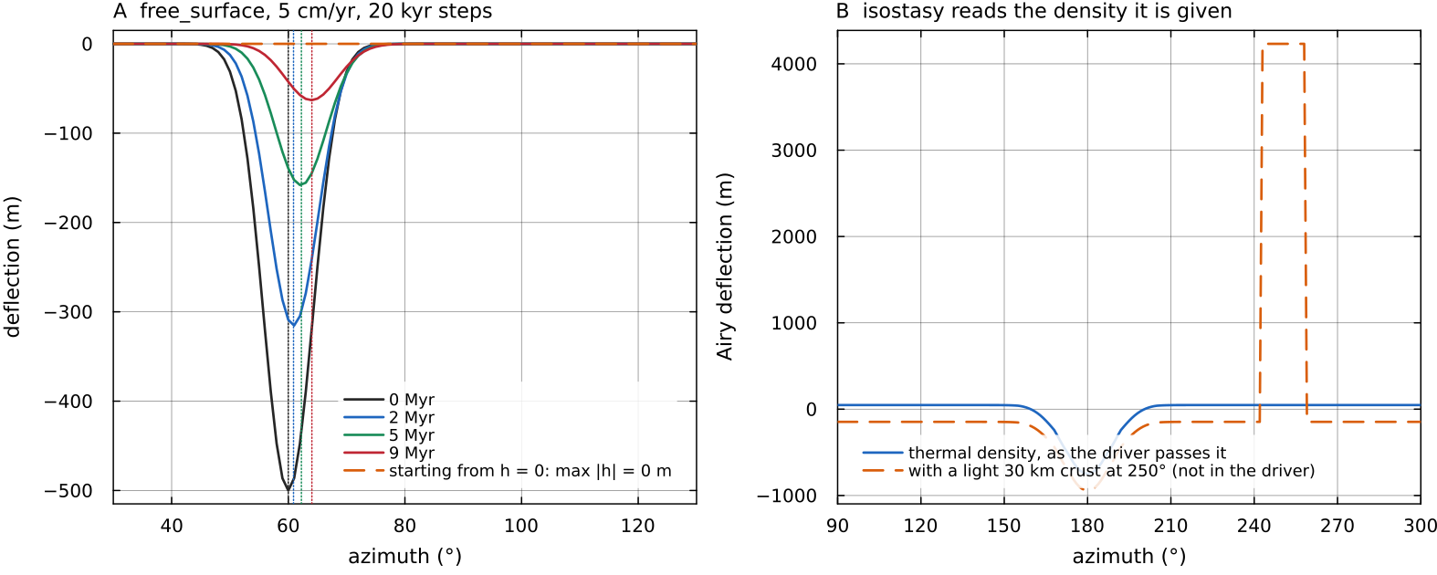
A: free_surface with a uniform 5 cm/yr surface flow and 20 kyr steps on a 64 × 360 annulus, starting from a 500 m depression; dotted lines mark where the flow alone would carry its centre. The deflection moves downstream and decays, because the stabilisation divisor (1.0045 per step here) damps it by a factor e every 4.5 Myr at this speed and cell size. Started from $h=0$, the tracker stays at zero. B: isostasy on the thermal density the driver passes, and on the same field with a 30 km crust 500 kg/m³ lighter added by hand; the driver never supplies the second, so compositional relief does not appear in the deflection. Script: docs/scripts/fig_free_surface_sections.jl.

Configuration

field	default	meaning
cfg.useStickyAir	false	weak air layer inside the domain
cfg.airThickness, cfg.airViscosity, cfg.airDensity	80 km, ${10}^{18}$ Pa s, 1.0	air layer
cfg.useFreeSurface	false	kinematic deflection tracker
cfg.freeSurfaceStabilization, cfg.freeSurfaceMaxDrop	0.5, 50 km	tracker stabilisation and clamp
cfg.useIsostasy, cfg.isostaticMode	false, "Airy"	isostatic deflection
cfg.isostaticDepth_km, cfg.isostaticTau_yr	100, 3000	compensation depth, relaxation time
cfg.flexuralRigidity, cfg.elasticThickness_km	0, 30	plate rigidity (flexural mode)

Where in the code

What	File, function
sticky air	utils/sticky_air.jl: apply_sticky_air!, sticky_air_mask
kinematic tracker, 2-D and 3-D	physics/free_surface.jl: free_surface
isostasy, 2-D and 3-D	physics/isostasy.jl: isostasy
calls and the top-cell temperature correction	main_SphCon.jl, steps 6, 7 and 13

Key references

• Schmeling, H. et al. (2008). A benchmark comparison of spontaneous subduction models: towards a free surface. PEPI 171, 198-223. doi:10.1016/j.pepi.2008.06.028

• Crameri, F. et al. (2012). A comparison of numerical surface topography calculations in geodynamic modelling: an evaluation of the "sticky air" method. GJI 189, 38-54. doi:10.1111/j.1365-246X.2012.05388.x

• Kaus, B. J. P., Mühlhaus, H. & May, D. A. (2010). A stabilization algorithm for geodynamic numerical simulations with a free surface. PEPI 181, 12-20. doi:10.1016/j.pepi.2010.04.007

• Turcotte, D. L. & Schubert, G. (2002). Geodynamics, 2nd ed., chapter 3.

• Haskell, N. A. (1935). The motion of a viscous fluid under a surface load. Physics 6, 265-269. doi:10.1063/1.1745329

• Hager, B. H., Clayton, R. W., Richards, M. A., Comer, R. P. & Dziewonski, A. M. (1985). Lower mantle heterogeneity, dynamic topography and the geoid. Nature 313, 541-545. doi:10.1038/313541a0

• Zhong, S., Gurnis, M. & Moresi, L. (1996). Free-surface formulation of mantle convection, I. Basic theory and application to plumes. GJI 127, 708-718. doi:10.1111/j.1365-246X.1996.tb04049.x

• Parsons, B. & Sclater, J. G. (1977). An analysis of the variation of ocean floor bathymetry and heat flow with age. JGR 82, 803-827. doi:10.1029/JB082i005p00803

• Hoggard, M. J., White, N. & Al-Attar, D. (2016). Global dynamic topography observations reveal limited influence of large-scale mantle flow. Nature Geoscience 9, 456-463. doi:10.1038/ngeo2709

• Ford, P. G. & Pettengill, G. H. (1992). Venus topography and kilometer-scale slopes. JGR Planets 97, 13103-13114. doi:10.1029/92JE01085

• Simons, M., Solomon, S. C. & Hager, B. H. (1997). Localization of gravity and topography: constraints on the tectonics and mantle dynamics of Venus. GJI 131, 24-44. doi:10.1111/j.1365-246X.1997.tb00593.x

Further reading

• Turcotte, D. L. & Schubert, G. (2014). Geodynamics, 3rd edn. Cambridge University Press. doi:10.1017/CBO9780511843877. Isostasy, plate flexure and the viscous relaxation of topography at an introductory level.

• Watts, A. B. (2023). Isostasy and Flexure of the Lithosphere, 2nd edn. Cambridge University Press. doi:10.1017/9781139027748. Airy, Pratt and flexural compensation, elastic thickness and the response function in depth.

• Schubert, G., Turcotte, D. L. & Olson, P. (2001). Mantle Convection in the Earth and Planets. Cambridge University Press. doi:10.1017/CBO9780511612879. Dynamic topography and the geoid as consequences of mantle flow.

• Gerya, T. (2019). Introduction to Numerical Geodynamic Modelling, 2nd edn. Cambridge University Press. doi:10.1017/9781316534243. Numerical treatments of the top boundary, including sticky air and marker-based surface tracking.