Temperature transport and time stepping

The time loop is main_SphCon in main_SphCon.jl. Each step solves Stokes for the current buoyancy and viscosity, picks the step size from the new velocity, moves the markers, then advances temperature by advection, heating and diffusion. This page covers the loop order, where temperature is stored, the advection and diffusion schemes, and the step-size control.

Step order

The numbered blocks in the loop body run in this order:

#	Block	Main calls
1	markers to grid	markers_to_grid
2	viscosity	composite_rheology (or the simpler laws)
3	melting, piles, basalt	melt_phase, basalt_evolution!
4	buoyancy (and the Yang-frame buoyancy in 3-D)	compute_buoyancy
5	Stokes, inside the Picard loop	see Solvers
6, 7	free surface, isostasy (optional)	free_surface
8	strain rate	compute_strain_rate
9	grain size (optional)	evolve_grain_size!
10, 11	time step, core-mantle boundary	compute_timestep, cmb_heat_flux
12	advect markers, then reseed every remeshEvery steps	advect_markers!, reseed_markers!
13	temperature: advection, sources, diffusion, hand-back	below
14 to 20	diagnostics, log, VTK, figures, checkpoint, NaN stop, time cap	diagnostics_row, save_vtu

The step size is chosen after the Stokes solve, from the velocity that will actually be used to advect, and that same $\mathrm{\Delta }t$ moves markers and temperature.

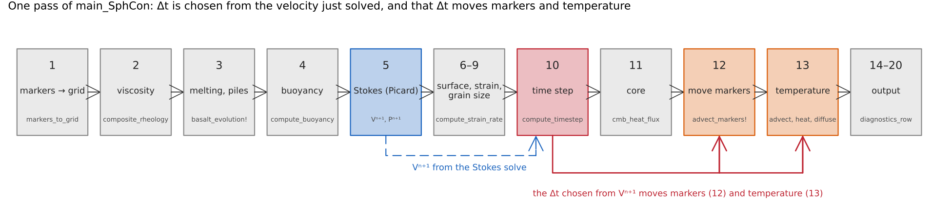
The numbered blocks of main_SphCon in the order of the table, with the function each one calls. The velocity of the Stokes solve (block 5) sets the step size in block 10, and that same $\mathrm{\Delta }t$ advects the markers (block 12) and the temperature (block 13). Schematic; the boxes carry the function names of the loop. Script: docs/scripts/fig_numerics_time_stepping_sections.jl.

Where temperature lives

Run	Temperature carried by	Grid temperature before diffusion	Advection
2-D, cfg.temperatureOnGrid = false (default)	markers	projection of marker $T$	marker RK4
2-D, cfg.temperatureOnGrid = true	grid	finite-volume advection of last step's grid $T$	advect_temperature_2d (cfg.tempAdvectionScheme)
3-D, Yin patch	markers	projection of marker $T$	marker RK4
3-D, Yang patch	grid	first-order upwind	advect_temperature_3d_upwind!

In the marker mode, diffusion and heating are solved on the grid and only the increment goes back to the markers, conservatively (see Markers). In the grid mode the markers carry composition only, and their temperature is set from the grid each step so marker-based physics such as melting can still read it.

Grid temperature with tracers for composition is the arrangement described by Tackley (2008); temperatureOnGrid = true selects it. The marker mode keeps the energy step exact through measure-scaled delivery and needs sub-grid diffusion to stay stable. On the Hernlund & Tackley (2008) isoviscous case at Ra = ${10}^5$, $N_r$ = 64, the two modes gave the same Nusselt number (8.97 on the grid with TVD, 8.88 on markers), so the choice of mode does not set that result.

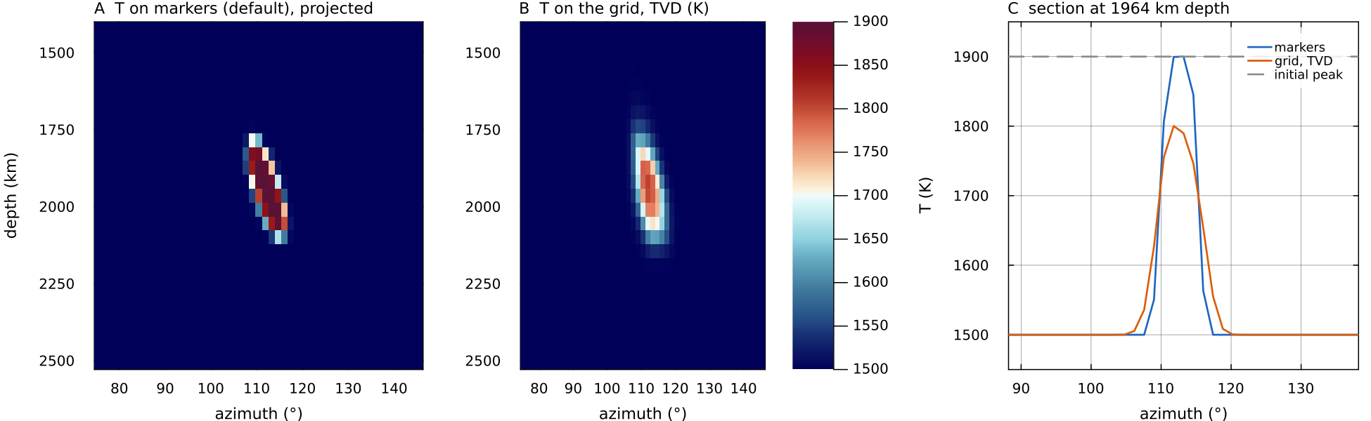
A 400 K warm disc, 350 km across, carried for 150 CFL steps through one fixed two-cell Stokes flow on a $64\times 256$ annulus without diffusion, once on the markers of init_markers (advect_markers!, then markers_to_grid) and once on the grid with advect_temperature_2d_tvd!. The marker field keeps its 1900 K peak and sharp edges; the TVD field loses about 100 K of peak to numerical diffusion and widens by a cell on each side. Script: docs/scripts/fig_numerics_time_stepping_sections.jl.

Advection on the grid

Both 2-D schemes (advect_temperature_2d_upwind!, advect_temperature_2d_tvd! in utils/advect_temperature.jl) are explicit finite-volume updates that use the same discrete divergence as the continuity rows of the Stokes assembly ($r^m$-weighted radial faces, $1/(r\mathrm{\Delta }\theta )$ in angle), and evaluate the advective form

$$T_c^{n+1}=T_c^n-\mathrm{\Delta }t[\mathrm{\nabla }\cdot (\mathbf{V}T{)}_c-T_c^n(\mathrm{\nabla }\cdot \mathbf{V}{)}_c],$$

so a uniform field stays exactly uniform whatever the discrete divergence of $\mathbf{V}$. The bracket is divided by the exact cell measure $(r_{F,i+1}^{m+1}-r_{F,i}^{m+1})/(m+1)$ rather than the midpoint $r_C^m\mathrm{\Delta }r$ (the whole increment is rescaled by their ratio, so the divergence stays a multiple of the continuity residual), and the fluxes therefore telescope in the measure of cell_measure and the energy diagnostics: an interior flow changes $\sum _c{T}_c{V}_c$ by round-off only. The 3-D versions do the same with the spherical metric factors $(1/r^2){\partial }_r(r^2{V}_{r}T)$ and $(1/(r\sin \theta )){\partial }_{\theta }(\sin \theta V_{\theta }T)$ (tests/test_advection_consistency.jl checks that a uniform field stays uniform).

The TVD scheme reconstructs each face value from the upwind cell with the van Leer limiter,

$$T_{\text{face}}=T_{\text{up}}+\frac{1}{2}\psi (\rho )(T_{\text{down}}-T_{\text{up}}),\psi (\rho )=\frac{\rho +|\rho |}{1+|\rho |},$$

where $\rho$ is the ratio of consecutive gradients (_vanleer, _slope_ratio). Because $\psi \le 2$, each face value stays between its two neighbouring cell averages, so the scheme adds no new extrema. Radial ghosts reflect the wall value, $T_{\text{ghost}}=2T_{\text{bc}}-T_{\text{wall cell}}$, and that same ghost is the second neighbour of the first interior cells (2 and $N_r-1$), so both cells next to an interior face reconstruct it with one stencil and its flux is counted once.

Use TVD, not upwind

cfg.tempAdvectionScheme defaults to "upwind", which is first order. Tackley (2008) reports that "the order of the advection scheme makes more difference than the number of cells", with this table (tetrahedral pattern, Ra = 7000, reference Nu = 3.4949):

Cells	Advection order	Nu	Reference Nu
24 576	1	3.62	3.4949
24 576	2	3.49	3.4949
196 608	1	3.57	3.4949
196 608	2	3.48	3.4949

Second order on the coarse grid beats first order on eight times the cells. In MILEVA, advecting a $\cos 4\theta$ pattern once around the annulus on a $16\times 256$ grid leaves about half of its amplitude with upwind while TVD keeps all of it, neither overshooting (figure below). Numerical diffusion acts as extra heat transport and raises the Nusselt number. Set cfg.tempAdvectionScheme = "TVD" whenever temperatureOnGrid = true. In the same benchmark run the TVD path showed a budget residual of +0.011, slightly larger than the marker path.

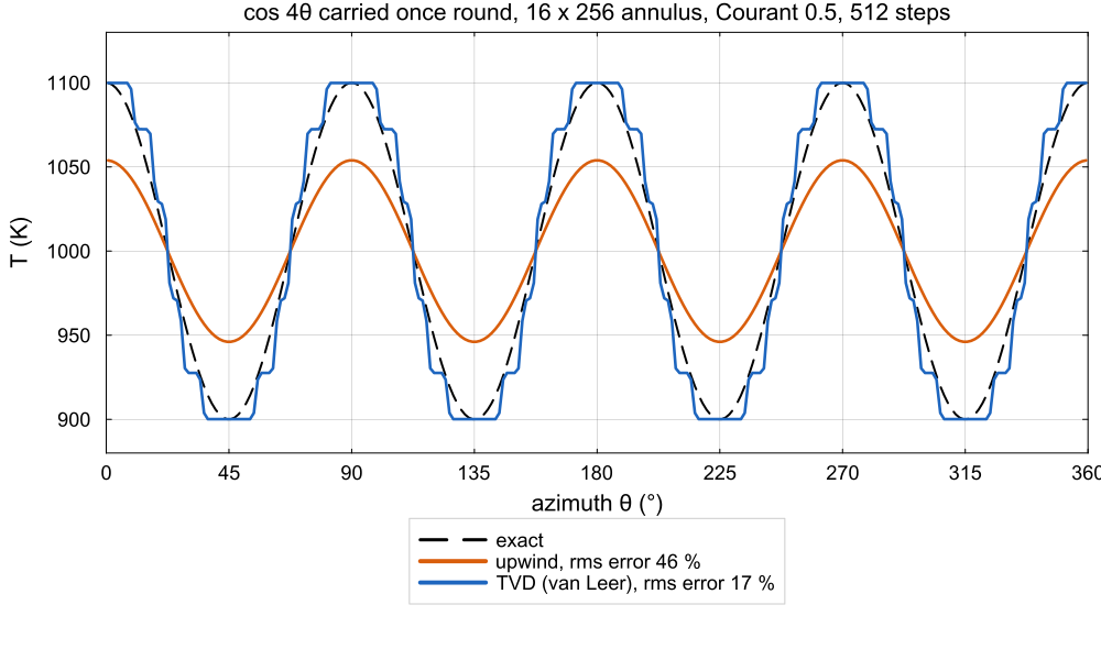
A $\cos 4\theta$ temperature pattern carried once round a $16\times 256$ annulus by rigid rotation at Courant number 0.5, with advect_temperature_2d_upwind! and advect_temperature_2d_tvd!. Upwind loses about half the amplitude to numerical diffusion; TVD keeps the peaks without overshoot, at the cost of small terraces on the flanks from the limiter.

In main_SphCon the 3-D Yang patch uses first-order upwind; the 3-D TVD scheme (advect_temperature_3d_tvd!) is what the 3-D example driver uses.

Diffusion and heating

diffuse_temperature (solvers/diffuse_temperature.jl) advances

$$\frac{\partial T}{\partial t}=\frac{1}{r^m}\frac{\partial }{\partial r}\left(r^m\kappa \frac{\partial T}{\partial r}\right)+\frac{\kappa }{r^2}\frac{{\partial }^{2}T}{\partial {\theta }^2}+\frac{H}{\rho c_p}$$

in 2-D (the 3-D form adds the spherical $\theta$ and $\phi$ terms). $H$ collects radiogenic heating and the volumetric sources passed in by the loop (latent heat, heat pipe, and the adiabatic and dissipation terms under ALA, which are carried together or not at all).

Conservative radial fluxes. The radial term is a flux difference across the two faces of each cell, with the face diffusivity and face radius inside the flux and division by the exact cell measure $\int r^{m}dr$ (_cell_vol). With a depth-dependent $\kappa$ this conserves energy where $\kappa (r){\mathrm{\nabla }}^{2}T$ does not; with constant $\kappa$ the two are algebraically identical.

Wall conditions at the faces. $T_{\text{cmb}}$ and $T_{\text{surf}}$ are imposed at the walls $R_{\text{in}}$ and $R_{\text{out}}$ through a half-cell ghost: the wall flux is $k(T_{\text{bc}}-T_{\text{wall cell}})/(\frac{1}{2}\mathrm{\Delta }r)$, and cells 1 and $N_r$ are ordinary flow cells. The discrete energy budget therefore closes exactly (see Energy budget).

Time discretisation.

Path	Default	Scheme
2-D, cfg.useImplicitTemp = true	yes	$\theta$-scheme $(I-\theta \mathrm{\Delta }tL)T^{n+1}=(I+(1-\theta )\mathrm{\Delta }tL)T^n+\mathrm{\Delta }tH$ with $\theta$ = cfg.implicitTheta (0.5, Crank-Nicolson; 1 is backward Euler)
2-D, useImplicitTemp = false		forward Euler
3-D, as called from the time loop	yes	forward Euler
3-D, implicit = true keyword		backward Euler, used by benchmark drivers

The 2-D operator $L$ and its LU factorisation are cached; the factor is reused while $\mathrm{\Delta }t$ is unchanged, which happens in fixed-step benchmarks but rarely under CFL control. Wall Dirichlet values enter the right-hand side as sources with the full $\mathrm{\Delta }t$, since they are constant over the step. After the solve, temperatures are clamped to $[max(T_{\text{surf}}-50,10),T_{\text{cmb}}+600]$ K; benchmarks in non-dimensional temperature must pass their own bounds in 3-D (clamp_lo, clamp_hi).

3-D explicit diffusion

The explicit 3-D update is stable for $\mathrm{\Delta }t\lesssim \mathrm{\Delta }{x}_{\text{min}}^2/(6\kappa )$; on a stretched grid with thin boundary cells keep cfg.dtMax below that bound. The 3-D stencil treats each patch's $\phi$-edges as periodic, so near those edges read temperatures from the peer patch.

In 3-D the patches are then coupled by the temperature Schwarz sweeps described on the Yin-Yang page.

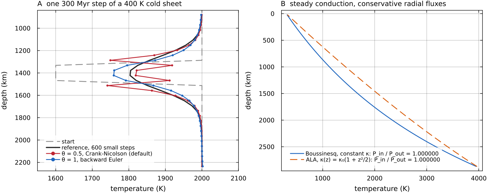
Left: one 300 Myr step of diffuse_temperature on a 180 km cold sheet ($N_r=64$, $\kappa \mathrm{\Delta }t/\mathrm{\Delta }{r}^2\approx 4.7$), against 600 small backward-Euler steps. Crank-Nicolson, the default, is second order but leaves an undamped cell-scale oscillation when the step is this large; backward Euler damps it at the cost of first-order accuracy. Under CFL control the diffusion number is usually far smaller. Right: steady conduction in the default shell with constant $\kappa$ and with the ALA diffusivity ${\kappa }_0(1+z^2/2)$. The conservative radial flux form passes the same power through both walls, boundary_power giving $P_{\text{in}}/P_{\text{out}}$ = 1.000000 in both cases, although the profiles differ. Script: docs/scripts/fig_numerics_time_stepping_sections.jl.

Step size

compute_timestep (utils/compute_timestep.jl) sets

$$\mathrm{\Delta }{t}_{\text{CFL}}=c\frac{\mathrm{\Delta }{x}_{\text{min}}}{max|\mathbf{V}|},\mathrm{\Delta }{x}_{\text{min}}=min(\mathrm{\Delta }{r}_{\text{min}},r_{\text{min}}\mathrm{\Delta }\theta ),$$

with $c$ = cfg.cflSafety (default 0.35) and, in 3-D, also $r_{\text{min}}\sin {\theta }_{\text{min}}\mathrm{\Delta }\phi$ in the minimum. The new step is

$$\mathrm{\Delta }t=min(\mathtt{\text{dtMax}},\mathrm{\Delta }{t}_{\text{CFL}},1.15\mathrm{\Delta }{t}_{\text{prev}}),$$

so it grows by at most 15 % per step; the first step is $\mathrm{\Delta }{t}_{\text{CFL}}$ clamped to $[\mathtt{\text{dtMin}},\mathtt{\text{dtMax}}]$ (defaults ${10}^6$ and $2\times {10}^{13}$ s). If the CFL step falls below dtMin, dtMin is used and a warning is logged (counter cfl_floor_hits()).

This is a global bound: the smallest cell anywhere against the fastest velocity anywhere. There is no diffusive limit, because the default 2-D diffusion is implicit. The 3-D bound uses $V_r$ and $V_{\theta }$ only, not $V_{\phi }$.

The velocity limiter (cfg.useVelocityLimit) rescales velocity and pressure whenever $V_{\text{max}}$ exceeds a cap. It is off by default; with it off, an exceedance is only reported.

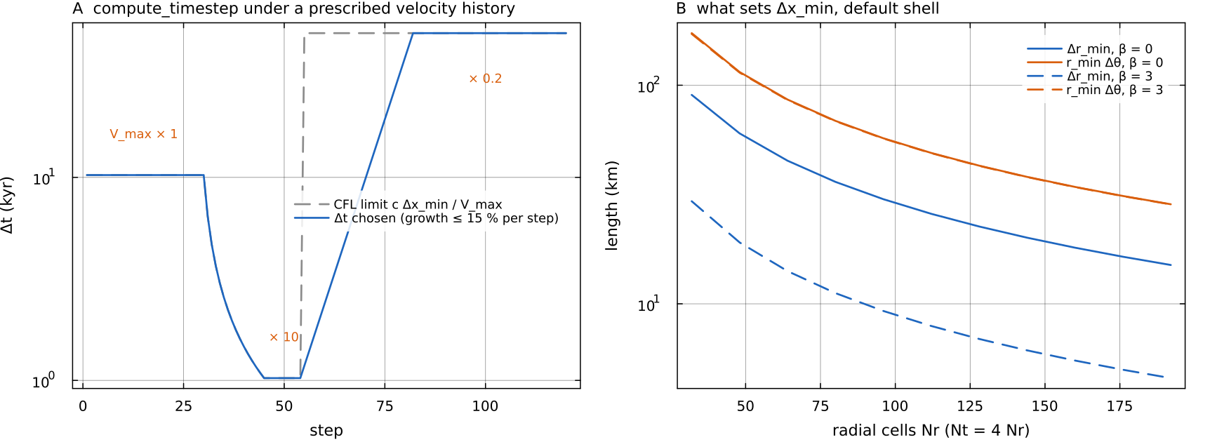
Left: compute_timestep called step by step while the velocity of a fixed $64\times 256$ flow is scaled by a prescribed factor (1, a ramp to 10, then 0.2). The step follows the CFL limit down at once, and after the velocity drops it grows by 15 % per step, taking 27 steps to reach the new limit. Right: the two lengths in $\mathrm{\Delta }{x}_{\text{min}}$ for the default shell; the radial cell width is the smaller at every $N_r$ with $N_t=4N_r$, and stretching with $\beta =3$ makes it about three times smaller still. Script: docs/scripts/fig_numerics_time_stepping_sections.jl.

Where in the code

Topic	File	Function
Time loop	main_SphCon.jl	main_SphCon
Grid advection	utils/advect_temperature.jl	advect_temperature_2d, advect_temperature_2d_tvd!, advect_temperature_2d_upwind!, advect_temperature_3d_tvd!, advect_temperature_3d_upwind!
Diffusion	solvers/diffuse_temperature.jl	diffuse_temperature, _solve_crank_nicolson, _solve_explicit
Step size	utils/compute_timestep.jl	compute_timestep, cfl_floor_hits
Tests	tests/	test_advection_consistency.jl, test_diffusion.jl, test_conduction_conservation.jl, test_nusselt_conduction.jl