Architecture

MILEVA is a flat-include research code: there is no package module and no using MILEVA. include/mileva.jl includes every source file into Main in dependency order, main_SphCon.jl defines the time loop, and a run is a script that includes both, edits the configuration and calls main_SphCon. Tests, the benchmark driver and the example scripts load the same graph.

There are four ways in:

Entry point	Loads	Time loop
a self-contained run script (see Getting started)	using Plots, include/mileva.jl, main_SphCon.jl	main_SphCon
benchmarks/hernlund_tackley_annulus.jl	the same	main_SphCon
run_mileva.jl <param.jl>	include/mileva.jl, main_SphCon.jl, then the parameter file into the pre-built cfg, mat, temp	main_SphCon (loads Plots first itself)
bin/run_mpi.jl <param.jl>	its own include list, including the distributed solver files	its own 2-rank loop

Include graph

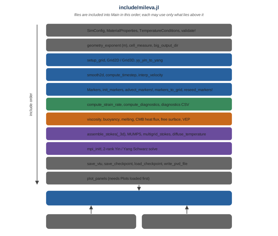
The layers of include/mileva.jl in include order, with the main entry points of each. main_SphCon.jl sits on top of the whole graph, and run scripts, the benchmark driver and the test runner all load the same graph.

include/mileva.jl loads, in this order; a file may use anything defined above it and nothing below:

Layer	Files (in order)	Provides
stdlib	SparseArrays, LinearAlgebra, Statistics, Random, Dates, Printf
config	config/SimConfig.jl, MaterialProperties.jl, TemperatureConditions.jl	the three @kwdef mutable structs, validate!, disp_summary, R_GAS
geometry	utils/geometry.jl	geometry_exponent(cfg) (the radial measure exponent $m$), cell_measure, cell_areas, surface_measure, big_output_dir
grid	utils/setup_grid.jl	Grid2D/MutableGrid2D, Grid3D/MutableGrid3D, setup_grid, the Kageyama and Sato transforms yy_yin_to_yang, yy_yang_to_yin
basic utils	utils/smooth2d.jl, compute_timestep.jl, interp_velocity.jl	smoothing, compute_timestep (CFL), velocity interpolation
markers	markers/init_markers.jl, advect_markers.jl, markers_to_grid.jl, interp_grid_to_markers.jl, subgrid_diffusion.jl, reseed_markers.jl	Markers, init_markers, advect_markers!, markers_to_grid, MarkerScatterWS, interp_grid_to_markers!, delivery_scale, subgrid_temperature_correction!, reseed_markers!
diagnostics	utils/compute_strain_rate.jl, compute_diagnostics.jl, diagnostics_csv.jl	compute_strain_rate, compute_diagnostics, lid_mobility_diagnostics, boundary_power, MeltLedger, the CSV writer
physics	physics/compute_viscosity.jl, composite_rheology.jl, compressibility.jl, compute_buoyancy.jl, melt_phase.jl, basalt_evolution.jl, surface_diagnostics.jl, evolve_grain_size.jl, thermochemical_piles.jl, antisqueeze.jl, cmb_heat_flux.jl, free_surface.jl, isostasy.jl, viscoelastoplastic.jl, damage.jl	viscosity, buoyancy, melting and melt transport, CMB heat budget (cmb_heat_flux, cool_core), free surface, isostasy, VEP, damage
solvers	solvers/stokes_assembly.jl (2-D), stokes_assembly_3d.jl, solve_stokes_v2.jl, solve_stokes_mumps.jl, solve_stokes_amg.jl, then utils/yy_interp.jl, fk_viscosity.jl, arrhenius_viscosity.jl, viscosity_jumps.jl, drucker_prager.jl, radiogenic.jl, advect_temperature.jl, sticky_air.jl, then solvers/multigrid_stokes.jl, diffuse_temperature.jl	assemble_stokes, assemble_stokes_3d, the 2-D direct/MUMPS/AMG solvers, Yin-Yang Schwarz boundary values, multigrid_stokes (2-D and 3-D), diffuse_temperature
parallel	parallel/mpi_init.jl, mpi_comm.jl, yinyang_mpi.jl, solvers/multigrid_stokes_mpi.jl	mpi_init!, the 2-rank Yin/Yang Schwarz solve
I/O	utils/save_vtu.jl, save_checkpoint.jl, load_checkpoint.jl, write_pvd_file.jl, save_snapshot.jl	save_vtu (2-D and 3-D), save_checkpoint, load_checkpoint, markers_from_checkpoint, write_pvd_file
visualization	visualization/plot_panels.jl	plot_panels (2-D figure panels; needs Plots in Main at load time)

solvers/solve_stokes_mumps.jl calls MPI.Init() when it is included, so every MILEVA process is an MPI singleton. The distributed files (parallel/local_grid.jl, halo_3d.jl, distributed_temperature.jl, distributed_stokes_phaseb.jl, solvers/distributed_stokes_*.jl, stokes_assembly_3d_local.jl, solve_stokes_distributed.jl) are not in this graph; only bin/run_mpi.jl and the MPI tests include them.

solvers/stokes_assembly_3d.jl and solvers/stokes_assembly_3d_local.jl are structural mirrors (the second assembles only a rank's owned rows). Any physics term added to one must be added to the other; tests/test_assembly_3d_mirror.jl compares them on a single rank.

Core data structures

Configuration

SimConfig, MaterialProperties and TemperatureConditions are mutable keyword structs with defaults, edited in place by a run script and checked by validate!. Two rules are worth knowing before adding a field:

• validate!(cfg) refuses flags that are declared but not implemented (for example cfg.useAMR and cfg.useDruckerPrager) and the ambiguous geometry = "annulus", rather than letting them be silently inert. tests/test_config_matrix.jl asserts that.

• The three driver hooks in SimConfig are the extension points for driver-specific physics, so the generic loop does not grow per-project parameters:

  Hook	Called	Signature
  initialMarkerHook	once after init_markers, fresh starts only	hook(M, grid, cfg, mat, temp)
  markerStepHook	every step after marker advection, before reseeding	hook(M, r_prev, grid, cfg, step, time_s, dt)
  restartHook	once after a checkpoint is restored	hook(M, Tg, grid, cfg, time_myr)

  After the first and the last, _assert_marker_lengths checks that the hook left every marker vector the same length.

Grids (utils/setup_grid.jl)

setup_grid(cfg, temp) dispatches on cfg.dim. Both results are a thin mutable wrapper around an immutable grid, so that the one quantity that evolves, the CMB temperature grid.T_cmb, can change while everything else is read only. getproperty forwards every other field to grid.inner; MutableGrid = Union{MutableGrid2D, MutableGrid3D} is used in signatures that accept either.

Grid2D (spherical or cylindrical annulus; the mesh is the same, only the metric factors differ):

Field	Size	Meaning
r, rF	Nr, Nr+1	cell-centre and face radii
th, dth	Nt, scalar	cell-centre angles, uniform spacing $2\pi /N_t$
RR, TH	Nr × Nt	meshgrids of r and th
drVec, drFVec	Nr, Nr+1	cell widths and centre-to-centre spacings (non-uniform when cfg.amrStretchFactor > 0)
dr	scalar	the minimum cell width, kept for the CFL limit
D, R_in, R_out, T_surf	scalars	layer thickness, radii, surface temperature
Tcond	Nr × Nt	a conductive reference profile

grid.dr is the smallest cell

On a stretched radial grid grid.dr == minimum(grid.drVec). Operators that need the local width use grid.drVec[i] (or drFVec).

Grid3D (one Yin-Yang patch; both patches share it, Yang is the rotated copy): cell centres r, th in $[\pi /4,3\pi /4]$ and ph in $[-3\pi /4,3\pi /4]$; counts Nr, Nth = cfg.Nt, Nph = 3 Nth; widths drVec, dthVec, dphVec and their face spacings; and the infrastructure of the overlap treatment (δ_yy buffer, live_mask, compact_idx, live_cells for the minimum-overlap grid). All of it reduces to the plain rectangular patch with the defaults (δ_yy = 0, cfg.useMinOverlapGrid = false). See Yin-Yang grid.

Field arrays

main_SphCon holds the solution as plain arrays sized by cell_dims ((Nr, Nt) in 2-D, (Nr, Nth, Nph) in 3-D), with staggered velocities:

Array	2-D size	3-D size
Vr	(Nr+1) × Nt (radial faces)	(Nr+1) × Nth × Nph
Vt / Vth	Nr × Nt	Nr × (Nth+1) × Nph
Vph	unused	Nr × Nth × (Nph+1)
P, ETA, strainII, ...	Nr × Nt	Nr × Nth × Nph

Composition reaches the physics as a Dict{Symbol,Array} named C_comp with the keys :continent, :pile, :eps_acc, :basalt, :depletion (and :hpe when melting is on).

Markers (markers/init_markers.jl)

Struct-of-arrays Lagrangian tracers in Float64:

Field	Meaning
r, th, ph	position; th is the azimuth in 2-D and the Yin colatitude in 3-D, ph is empty in 2-D
T	temperature (K)
d	grain size (m)
C, pile, basalt, depletion	continent, thermochemical-pile, basalt and depletion fractions
eps_acc, erupt_time	accumulated strain; time basalt was last deposited at the surface
hpe	heat-producing-element concentration relative to primitive mantle, partitioned at melt extraction so $\sum w\mathrm{hpe}$ is conserved
volatile	passive concentration (ppm), advected and conserved, no feedback
w	persistent marker weight: area (2-D, m²) or volume (3-D, m³), set at initialisation, carried through advection, redistributed by reseeding. Every inventory is $\sum _m{w}_m{f}_m$
cstage, cmox, cmred, root0	per-parcel state written only by a driver's markerStepHook or initialMarkerHook; inert otherwise
dim	2 or 3

MARKER_VECTOR_FIELDS lists every per-marker vector. Anything that culls, subsets or appends markers must go through it (subset_markers!), because the hot loops are @inbounds and one array left behind desynchronises the set.

MarkerScatterWS (markers/markers_to_grid.jl) is the preallocated thread-local workspace of the marker-to-grid projection. Its field W keeps the accumulated marker measure per node from the last projection, which delivery_scale(grid, cfg, ws) turns into the factor cell measure / W that makes the hand-back of a grid increment to the markers exactly conservative. The factor is clamped to $[1/c,c]$ with $c$ = cfg.deliveryScaleMax (default 2), so a sparsely populated wall cell cannot hand a few markers several times the cell's increment; the energy a clamped node does not receive shows up in budget_resid, not in the velocity.

The time loop, step by step

main_SphCon(cfg, mat, temp) (main_SphCon.jl) validates and prints the configuration, creates the output directories, builds the grid (setup_grid) and the markers (init_markers, then initialMarkerHook), allocates the field arrays, optionally restores a checkpoint (cfg.resumeFrom), opens the log and diagnostics.csv, and then runs for step in start_step:cfg.maxSteps.

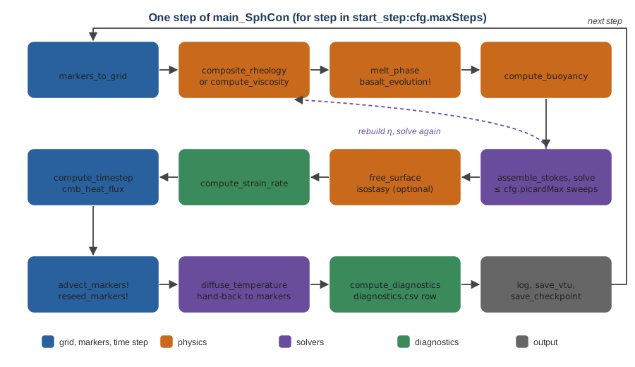
One pass through the loop body, numbered as the block comments in main_SphCon.jl. The dashed arrow is the Picard iteration of step 5, which rebuilds the viscosity from the new strain rate and solves again.

The numbers below are the block comments in the source:

1. Markers → grid. markers_to_grid projects T, grain size, continent, pile and accumulated strain to cell centres, with the reference adiabat as the fill for empty cells. With cfg.temperatureOnGrid (2-D), T instead comes from the grid array carried over from the previous step. Without melting, depletion is projected separately by project_marker_field_2d, so a driver-painted depletion reaches the grid.

2. Viscosity. Optional antisqueeze, then composite_rheology (if cfg.useCompositeRheology) or compute_viscosity plus the optional Frank-Kamenetskii law, depletion stiffening and crust factor, then viscoelastoplastic and the damage factor.

3. Melting and composition. melt_phase (melt fraction, phase id, latent heat), thermochemical_piles!, and basalt_evolution! (extraction, eruption and intrusion of melt, the heat-pipe sink, HPE partitioning; adds to the cumulative MeltLedger). Melting is skipped while dt == 0.

4. Buoyancy. compute_buoyancy, with the ALA/TALA adiabat from compressibility when cfg.compressibilityMode is not Boussinesq, and sticky air if enabled. 4b: in 3-D, the same for the Yang patch from its own temperature Tg_yang.

5. Stokes with the nonlinear iteration. Up to picard_max sweeps (cfg.picardMax, or 50 when a yield law is active and 1 otherwise) of: solve, remove the net rotation (2-D), recompute the strain rate, rebuild the viscosity (damped in log space by cfg.picardDamping), until the relative change in V_max is below cfg.picardTol. Non-convergence is counted and logged, never silent. The solver dispatch is in the table below. The velocity limiter only warns unless cfg.useVelocityLimit.

6. Free surface (free_surface) and 7. isostasy (isostasy), when on.

7. Strain rate. compute_strain_rate from the converged velocity; the accumulated strain is added to the markers with interp_grid_to_markers!.

8. Grain size. evolve_grain_size!.

9. Time step by compute_timestep (CFL, capped by cfg.dtMax), and

10. CMB: cmb_heat_flux or cmb_conductive_flux for the wall flux.

11. Advect markers with advect_markers! (RK4 by default, cfg.advectionScheme = "RK2" for midpoint), then markerStepHook. 12b. Reseeding every cfg.remeshEvery steps (reseed_markers!), conservative in composition and weight.

12. Temperature. Advection is either the marker projection or, with cfg.temperatureOnGrid, advect_temperature_2d. The volumetric sources (adiabatic and viscous terms, both or neither, gated by cfg.useShearHeating; latent heat; eruption heat) are summed into H_combined, and diffuse_temperature takes the conduction and heating step (Crank-Nicolson by default, with the Dirichlet wall values applied at the wall faces through a half-cell ghost). In 3-D the Yang temperature is advected and diffused alongside, with cfg.nTSchwarz rounds of wall exchange. On the marker path, the increment dT_corr (minus the sub-grid correction of subgrid_temperature_correction!) is handed back to the markers scaled by delivery_scale, which makes the transfer energy conserving wherever the scale is not clamped; marker T is then clamped to $[max(T_{\mathrm{surf}}-50,10),T_{\mathrm{cmb}}+600]$ K.

13. Diagnostics. compute_diagnostics (V_rms, Nu, ⟨T⟩, lid thickness), the resurfacing detector, surface diagnostics, lid mobility, and the energy bookkeeping: the wall power from boundary_powerand the internal power are accumulated every step with the diffusion solver's own time weighting, and with a cooling core (cmbHeatfluxMode = "parameterized", 2-D)cool_coredebits the core by the energy it delivered. A row goes todiagnostics.csv.

14. Log line.

15. VTK output (save_vtu, then write_pvd_file).

16. Figures (plot_panels, 2-D only) and the per-block timing table.

17. Checkpoint (save_checkpoint).

18. Stop on NaN or V_rms > 1e6 cm/yr.

19. Stop at cfg.maxTimeMyr when it is positive.

After the loop it prints the final state, the melt ledger and the timing averages, and returns the history (time, V_rms, Nu, ⟨T⟩, q_cmb, lid diagnostics, ...) merged with the final fields (Tg, Vr, Vt, and in 3-D Vph, the Yang solution and Tg_yang).

Stokes solver dispatch

Case	Routine	File
3-D, any solverType	multigrid_stokes(::MutableGrid3D, ...): FGMRES with an SCGS-smoothed V-cycle on each patch, Yin and Yang coupled by Schwarz iteration	solvers/multigrid_stokes.jl
2-D, "mumps"	solve_stokes_mumps (MUMPS multifrontal LU, factorisation cache)	solvers/solve_stokes_mumps.jl
2-D, "direct" (default)	solve_stokes_v2 (UMFPACK)	solvers/solve_stokes_v2.jl
2-D, "amg"	solve_stokes_amg (falls back to the direct solve whenever its tolerance is not met)	solvers/solve_stokes_amg.jl
2-D, "multigrid"	multigrid_stokes(::MutableGrid2D, ...) (SCGS V-cycle, Galerkin coarse operators)	solvers/multigrid_stokes.jl

All 2-D solvers share one assembly, assemble_stokes in solvers/stokes_assembly.jl, which factors the viscous operator as $L_{\mathrm{visc}}=RS$ with $S$ the constitutive law $\tau =2\eta \dot{\epsilon }$ and $R$ the discrete divergence, so $\mathrm{\nabla }\cdot (2\eta \dot{\epsilon })$ holds by construction. For 2-D production use "mumps": on the shared assembly it was 2.5× faster than UMFPACK at 32 × 96 and 20× faster at 96 × 288. See Discretization.

Where 2-D and 3-D differ in the loop

Item	2-D	3-D
Stokes	four backends	multigrid + Schwarz only
Net rotation removal	cfg.removeNetRotation (default on)	no effect
Temperature on the grid	optional (cfg.temperatureOnGrid)	Yin from markers; Yang a grid field (advect_temperature_3d_upwind!)
Cooling core debit	cool_core after each step	not applied in the loop
Panel figures	plot_panels	none

The MPI path does not run this loop. bin/run_mpi.jl has its own 2-rank time loop with a fixed viscosity and its own initial condition, so none of the steps above beyond the Stokes and temperature solves applies there. Unifying the two loops is outstanding work.