Boussinesq, TALA and ALA (2-D)

The same basally heated, isoviscous shell solved under the three formulations of the mass and energy equations that cfg.compressibilityMode offers, at three dissipation numbers. The page shows what each formulation changes in the flow and the temperature, and checks a property every steady compressible solution must have: the heat made by viscous dissipation equals the work done against the adiabatic term.

The three formulations

mode	mass balance	density in the heat capacity	adiabatic heating $-{\rho }_{\text{ref}}\alpha gT{v}_r$	viscous dissipation $\mathrm{\Phi }$
"Boussinesq"	$\mathrm{\nabla }\cdot \mathbf{v}=0$	${\rho }_0$	no	no
"TALA"	$\mathrm{\nabla }\cdot ({\rho }_{\text{ref}}\mathbf{v})=0$	${\rho }_{\text{ref}}(r)$	no	no
"ALA"	$\mathrm{\nabla }\cdot ({\rho }_{\text{ref}}\mathbf{v})=0$	${\rho }_{\text{ref}}(r)$	yes	yes

Under both anelastic modes the stress is the compressible deviator and the buoyancy is ${\rho }_{\text{ref}}g\alpha \delta T$, with $\delta T$ the lateral anomaly of $T-T_{\text{ad}}$. The two O(Di) heat terms are switched on together by cfg.useShearHeating; the driver sets it for ALA only. The full equations are in Governing equations.

The names are not King et al.'s

In King et al. (2010) the truncated anelastic liquid approximation (TALA) keeps adiabatic heating and dissipation and drops only the dynamic-pressure part of the buoyancy. MILEVA's ALA also has a buoyancy that depends on temperature alone, so MILEVA's ALA is the closer match to King et al.'s TALA. MILEVA's "TALA" is an anelastic model with the O(Di) heating switched off, a formulation that the published benchmarks do not cover. Use it to separate the effect of the reference density from that of the heat terms, as on this page, not as a physical model of a mantle.

The model

The shell of the other examples ($f=0.5495$, $D=1000$ km), free slip, isothermal walls at $T_{\text{surf}}=273$ K and $T_{\text{CMB}}=3273$ K, so $\mathrm{\Delta }T=3000$ K and $T_{\text{surf}}/\mathrm{\Delta }T=0.091$, the value of King et al. (2010). The dissipation number

$$Di=\frac{\alpha gD}{c_p},c_p=1250{\text{J kg}}^{-1}{\text{K}}^{-1}$$

is set through a constant expansivity, and the viscosity follows so that the surface Rayleigh number $\mathrm{Ra}={\rho }_{0}g\alpha \mathrm{\Delta }T{D}^3/(\kappa \eta )$ stays at ${10}^5$. With a Grüneisen parameter of 1 and the adiabat started at the surface temperature, the reference state is King et al.'s, $T_{\text{ad}}=T_{\text{surf}}{e}^{Diz/D}$ and ${\rho }_{\text{ref}}={\rho }_0{e}^{Diz/D}$: the density at the CMB is 1.28, 1.65 and 2.72 times the surface density at $Di$ = 0.25, 0.5 and 1.

parameter	value	where
grid	64 × 512, uniform in radius	ht_shell!
Ra	${10}^5$, from the surface density and expansivity	eta_for_Ra
$Di$	0.25, 0.5, 1 (Boussinesq uses the expansivity of $Di=0.5$)	second argument
$\alpha$	$3.19$, $6.37$, $12.7\times {10}^{-5}$ K⁻¹	cfg.alpha = Di c_p/(g D)
$\eta$	$3.1\times {10}^{22}$, $6.2\times {10}^{22}$, $1.2\times {10}^{23}$ Pa s
$\kappa$	${10}^{-6}$ m² s⁻¹, constant with depth	cfg.kappaDepthFactor = 0
Grüneisen parameter	1	cfg.gruneisen
initial condition	linear ramp, 6 warm cosine peaks of 60 K at the CMB, 3 K noise
run length	0.25 thermal diffusion times, 7922 Myr, about 25 000 steps	cfg.maxTimeMyr
output	VTK every 2000 steps, diagnostics.csv and the log every 500

cfg.kappaDepthFactor = 0 matters here. The default ALA diffusivity grows toward the CMB as $\kappa (1+0.5z^2)$ (with $z$ the normalised depth), which would make the anelastic runs differ from Boussinesq in a second way.

Results

The seven runs side by side over their first 873 Myr, same layout and colour scale as the still below. These are short preview runs of the same driver (3000 steps, a VTK frame every 60 steps), not the long runs behind the table; each panel shows the run's frame nearest to the common model time. Script: docs/scripts/render_compressible_anim.jl.

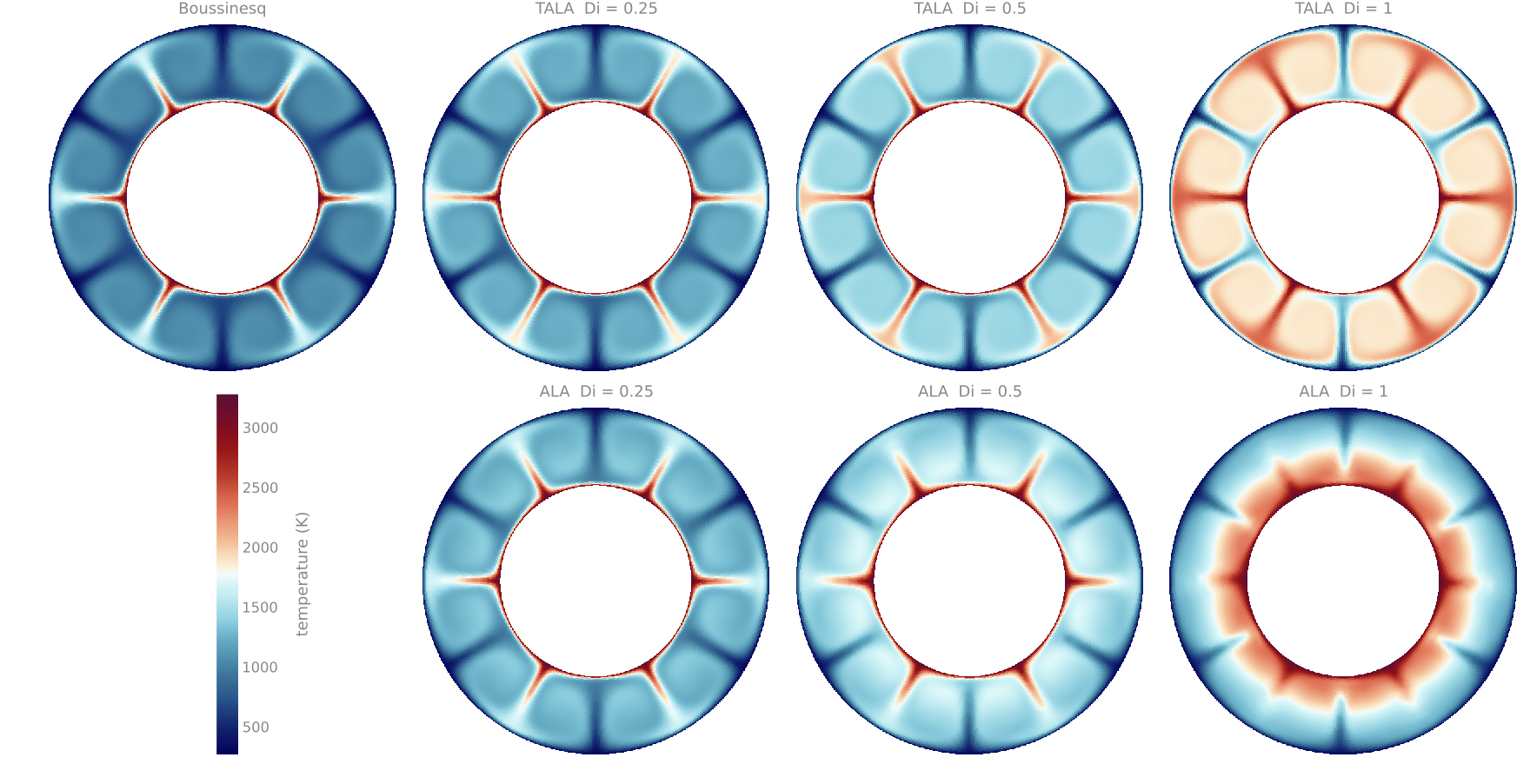
Temperature at the last VTK frame (about 7550 Myr) of the seven runs, on one colour scale. Top: Boussinesq and TALA at $Di$ = 0.25, 0.5, 1. Bottom: ALA at the same dissipation numbers. All seven keep the six upwellings of the seeded planform.

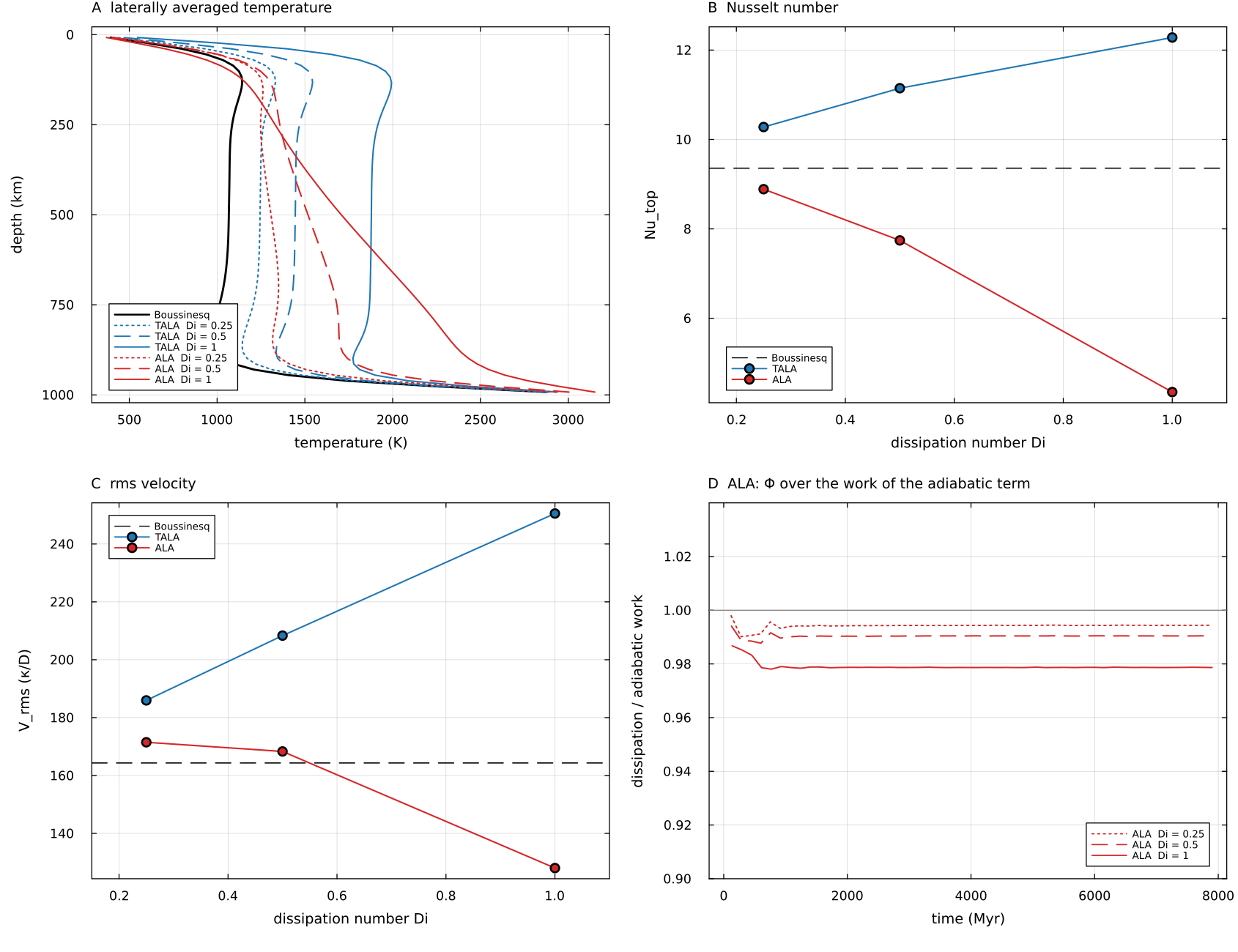
A: laterally averaged temperature, mean over the last five VTK frames (5000 to 7600 Myr). B, C: ${\mathrm{Nu}}_{\text{top}}$ and $V_{\text{rms}}$ against $Di$, Boussinesq dashed. D: viscous dissipation over the work of the adiabatic term in the three ALA runs, from the [H terms mW/m2] lines of the run log. Script: docs/scripts/fig_compressible.jl.

Means over the last third of the rows of diagnostics.csv (5300 to 7900 Myr). Over that window ${\mathrm{Nu}}_{\text{top}}$ varies by 1 to 2 % in every run, so the flows are statistically steady:

mode	Di	Nu_top	Nu_bot	V_rms (κ/D)	q_surf (mW m⁻²)	⟨T⟩ (K)	budget_resid	Φ / adiabatic work
Boussinesq	(0.5)	9.36	9.33	164	63.6	1063	−0.0001
TALA	0.25	10.28	10.25	186	81.0	1231	−0.0010
TALA	0.5	11.15	11.13	208	101.2	1421	−0.0001
TALA	1	12.28	12.27	251	145.9	1834	−0.0003
ALA	0.25	8.89	8.87	172	70.0	1259	−0.0004	0.994
ALA	0.5	7.74	7.74	168	70.3	1425	−0.0005	0.990
ALA	1	4.35	4.39	128	51.6	1556	+0.0009	0.979

The numbers are also in docs/src/media/examples_compressible.csv.

The checks. In every run ${\mathrm{Nu}}_{\text{top}}$ and ${\mathrm{Nu}}_{\text{bot}}$ agree to better than 1 %, and the energy budget residual stays at or below 0.001 of the surface power. Under ALA the dissipation equals the work of the adiabatic term to 0.6, 1.0 and 2.1 % at $Di$ = 0.25, 0.5 and 1 (panel D). In the continuous equations the two are equal in any steady state, because the anelastic mass balance makes $\int {\rho }_{\text{ref}}{v}_r$ vanish on every shell, so the adiabatic work equals the buoyancy work, which equals the dissipation. The remaining gap is therefore discretisation error at 64 × 512. It grows with $Di$; a resolution study has not been run.

ALA: compressibility slows the flow. The interior follows the adiabat. Between 300 and 700 km depth its temperature rises at 0.24, 0.68 and 1.66 K/km, which is 73, 89 and 97 % of the adiabatic gradient $DiT/D$ (0.33, 0.76 and 1.72 K/km at the mid-depth temperature). That adiabatic rise uses up part of the 3000 K across the shell, so less temperature difference is left to drive the flow, and a rising parcel cools as it expands. Nusselt number, velocity and surface heat flow all fall as $Di$ grows: ${\mathrm{Nu}}_{\text{top}}$ drops from 9.36 (Boussinesq) to 4.35 at $Di=1$. The same trend, convection weakening with $Di$, is what King et al. (2010) report for their anelastic cases in a Cartesian box. Their numbers do not apply to the annulus, so they are not compared here.

TALA: the reference density alone does the opposite. Without the two heat terms the interior stays isothermal, as in Boussinesq: the gradient between 300 and 700 km is −0.05 K/km at $Di=1$, against an adiabatic 1.88. The only effect left is the reference density. It rises with depth, so the buoyancy ${\rho }_{\text{ref}}g\alpha \delta T$ and the conductivity ${\rho }_{\text{ref}}{c}_p\kappa$ are both larger at depth than the surface values that define Ra. The deep mantle therefore convects as if Ra were higher, and ${\mathrm{Nu}}_{\text{top}}$, $V_{\text{rms}}$ and the interior temperature all rise with $Di$. This is why MILEVA's TALA is not a model of a compressible mantle: dropping the heat terms removes the effect that matters most.

Nusselt numbers are measured against the conductive state of each run's own operator. Under ALA and TALA that conductive profile depends on ${\rho }_{\text{ref}}$, so Nu values at different $Di$ are not ratios to the same reference. Compare the surface heat flow $q_{\text{surf}}$ as well.

Compared with published work

None of the studies below uses this shell, so they are compared by the direction of each effect, not by its size.

behaviour	published	MILEVA
vigour of convection with adiabatic heating and dissipation (fixed Ra, Di raised)	lower: "for the Di = 1.0 cases the vigour of convection is reduced", King et al. (2010), 2-D Cartesian box, for their TALA and ALA	lower: Nu, $V_{\text{rms}}$ and $q_{\text{surf}}$ fall from Di = 0.25 to 1 under ALA
dissipation against the work of the adiabatic term	in balance in a steady state; across the codes the imbalance grows with Di up to 1.25 and then shrinks (King et al. 2010, their TALA at Ra = 10⁵)	gap of 0.6, 1.0 and 2.1 % at Di = 0.25, 0.5 and 1
does the form of the mass balance matter?	little: the anelastic, isentropic-compression and projected-density mass balances, all with adiabatic heating, change the heat flow by about a percent (Gassmöller et al. 2020)	Boussinesq and TALA differ by 10 to 30 %, but they also differ in the density of the buoyancy and the conduction terms, which the comparison above holds fixed
planform in a spherical geometry	fewer upwelling plumes and irregular, time-dependent patterns as compressibility grows, when the superadiabatic temperature drop is small against the adiabatic temperature (Bercovici, Schubert & Glatzmaier 1992, 3-D spherical shell)	not tested: all seven runs keep the six upwellings of the seeded planform
density stratification with the heat terms off (MILEVA's TALA)	no published counterpart found; the extended Boussinesq approximation of King et al. is the complementary split, heat terms on and density constant	faster: Nu, $V_{\text{rms}}$ and interior temperature rise with Di

So MILEVA's ALA behaves as published compressible models do: adding adiabatic heating and dissipation slows the flow and lowers the heat flow. The speed-up under MILEVA's TALA has no published reference. It is consistent with the Gassmöller et al. result above: the mass balance alone changes little, so the speed-up comes from the reference density raising the buoyancy and the conductivity at depth while no adiabatic cooling acts against it.

Running it

export GKSwstype=nul
julia --project=. -t 2 examples/annulus_compressible_2d.jl ALA 0.5 1e5 64

Arguments are mode Di Ra Nr; mode is Boussinesq, TALA or ALA. Output goes to output/examples/compressible_ALA_Di0.5_Ra1e+05_N64/. At the end the driver prints the window means of the table and, under ALA, the adiabatic and dissipation powers with their ratio.

Each run took 5 to 8 hours of wall time on a 10-core Mac mini with four of them sharing the machine. Shorten a run with MILEVA_MAXTIME_MYR or MILEVA_MAXSTEPS. The figures come from

julia --project=. docs/scripts/fig_compressible.jl output/examples

References

Bercovici, D., Schubert, G. & Glatzmaier, G. A. (1992). Three-dimensional convection of an infinite-Prandtl-number compressible fluid in a basally heated spherical shell. J. Fluid Mech. 239, 683-719. doi:10.1017/S0022112092004580

Gassmöller, R., Dannberg, J., Bangerth, W., Heister, T. & Myhill, R. (2020). On formulations of compressible mantle convection. Geophys. J. Int. 221, 1264-1280. doi:10.1093/gji/ggaa078

King, S. D., Lee, C., van Keken, P. E., Leng, W., Zhong, S., Tan, E., Tosi, N. & Kameyama, M. C. (2010). A community benchmark for 2-D Cartesian compressible convection in the Earth's mantle. Geophys. J. Int. 180, 73-87. doi:10.1111/j.1365-246X.2009.04413.x