Staggered finite volumes in the annulus

MILEVA discretises the Stokes equations on a staggered (marker-and-cell) grid in polar coordinates $(r,\theta )$ for 2-D runs, and in spherical coordinates $(r,\theta ,\phi )$ on each Yin-Yang patch for 3-D runs (see Yin-Yang grid). Velocities live on cell faces, pressure, temperature, viscosity and composition at cell centres. The 2-D assembly is assemble_stokes in solvers/stokes_assembly.jl; the 3-D assembly is assemble_stokes_3d in solvers/stokes_assembly_3d.jl. Every 2-D Stokes solver (direct, MUMPS, BiCGSTAB, multigrid) calls the same assembly and differs only in how it solves the resulting matrix, so the discrete problem does not depend on the solver choice.

Geometry: one exponent

The meshes themselves, and the four geometries MILEVA runs on (2-D spherical and cylindrical annulus, 3-D chunk and Yin-Yang sphere), are drawn on Grids and geometries.

Both 2-D geometries share the same mesh. They differ only in how the area of a shell grows with radius, $A(r)\propto r^m$, and geometry_exponent(cfg) in utils/geometry.jl returns that exponent:

cfg.geometry	$m$	Measure	Meaning
"spherical_annulus" (default)	2	$r^{2}drd\theta$	equatorial slice of a spherical shell (Hernlund & Tackley 2008)
"cylindrical_annulus"	1	$rdrd\theta$	cross-section of an infinite cylinder

Every operator that needs a radial metric asks for $m$ instead of hard-coding a power of $r$: the continuity divergence $(1/r^m){\partial }_r(r^m{V}_r)$, the viscous stress divergence, the temperature diffusion and advection operators, the cell measures used by markers and diagnostics, and the conductive baseline of the Nusselt number. The bare spelling "annulus" is refused by validate! in config/SimConfig.jl, because the two geometries differ by a factor of about 1.95 in the core-to-surface area ratio for a Venus-sized body and a silent choice changes the answer.

Use the spherical annulus

The spherical annulus (Hernlund & Tackley 2008) gives the core-mantle boundary the area ratio of a sphere, and published reference values exist for it (Hernlund & Tackley 2008; the "Annulus" column of Fleury et al. 2024). All examples and benchmarks in this documentation use it. The cylindrical setting is kept so older results can be reproduced.

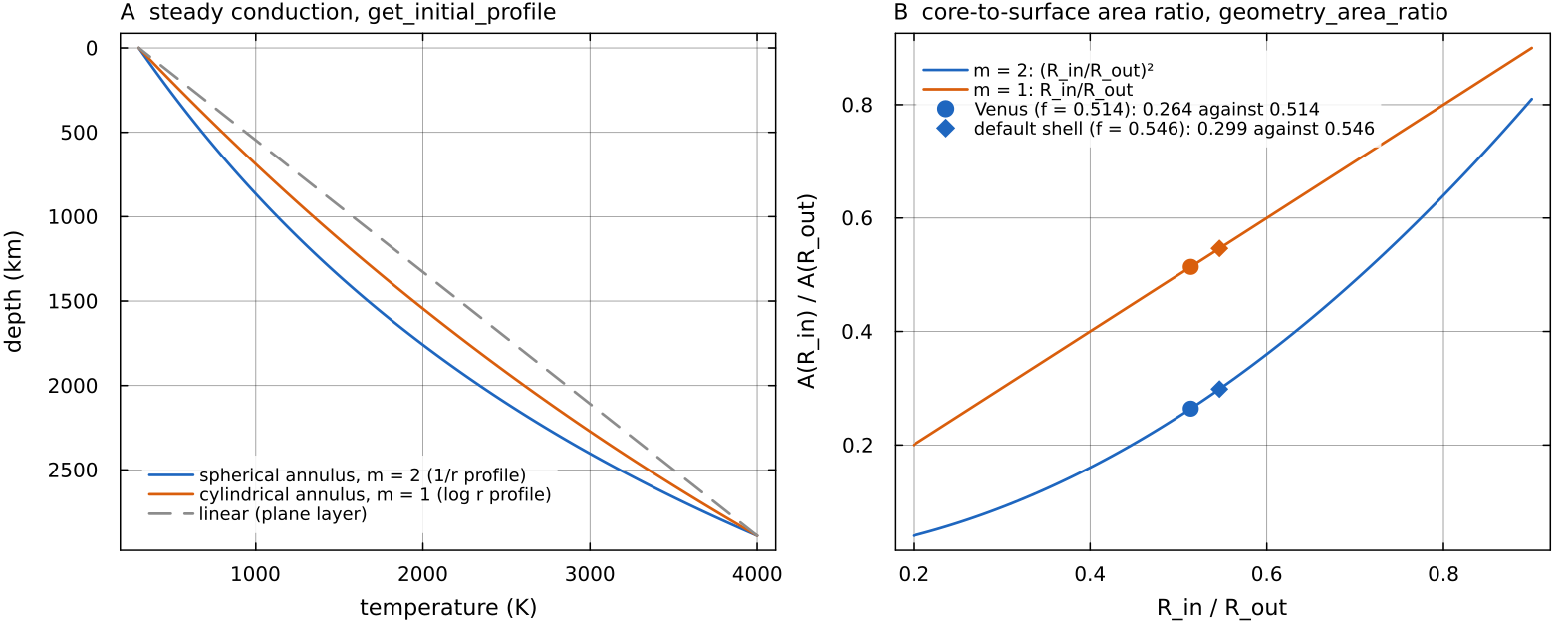
What the one exponent changes. Left: the steady conductive temperature that get_initial_profile returns for the default shell with $m=2$ (a $1/r$ profile) and $m=1$ (a logarithm), against a straight line; at mid-depth they differ by about 270 K. Right: geometry_area_ratio against $R_{\text{in}}/R_{\text{out}}$; for Venus the core-mantle boundary has 0.264 of the surface area in the spherical annulus and 0.514 in the cylinder. Script: docs/scripts/fig_numerics_discretization_sections.jl.

Staggered layout (2-D)

Field	Array size	Location
$V_r$	$(N_r+1)\times N_t$	radial faces $r_{F,i}$, cell-centre angles
$V_{\theta }$	$N_r\times N_t$	angular faces, cell-centre radii
$P$, $T$, $\eta$, $C$	$N_r\times N_t$	cell centres

The angle $\theta$ is periodic over $2\pi$ with $\mathrm{\Delta }\theta =2\pi /N_t$. The unknowns are ordered row-major in $\theta$ (v_idx(i,j) = (i-1)*Nt + j), which keeps the periodic wrap-around connection at a bandwidth of about $N_t$ rather than $N_r{N}_t$; the comment in assemble_stokes records that this reduced LU fill-in from about $79\times {10}^6$ to about ${10}^6$ entries at its test size.

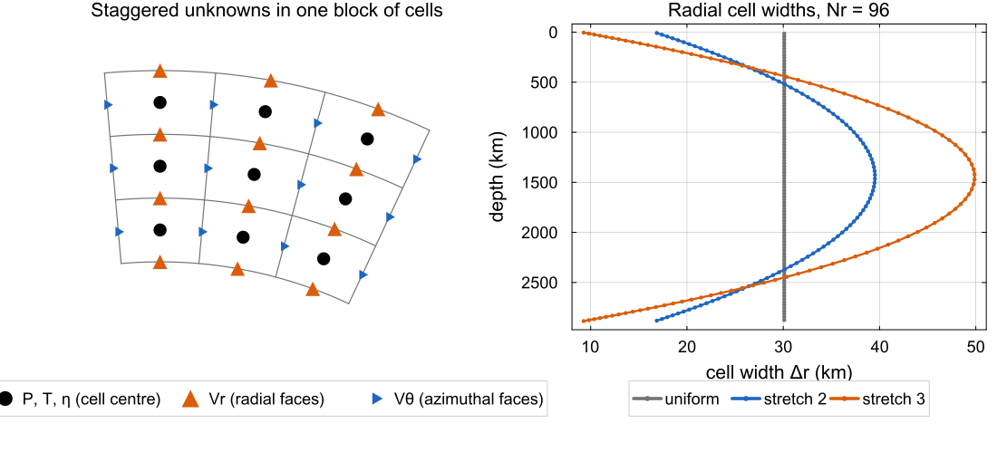
Left: where the unknowns of one block of cells sit, pressure, temperature and viscosity at cell centres, $V_r$ on the radial faces and $V_{\theta }$ on the azimuthal faces. Right: the radial cell widths setup_grid returns for the default shell at $N_r=96$, uniform and with amrStretchFactor 2 and 3, which refine both boundary layers at the expense of the mid-mantle (see Radial grid stretching).

Non-dimensional, row-equilibrated system (2-D)

assemble_stokes builds the system in non-dimensional variables, with the layer thickness $D=R_{\text{out}}-R_{\text{in}}$, the thermal diffusivity $\kappa$ and the median viscosity ${\eta }_{\text{ref}}$ of the current field as scales:

$$\overline{r}=r/D,\overline{V}=VD/\kappa ,\overline{P}=P{D}^2/({\eta }_{\text{ref}}\kappa ),\overline{\eta }=\eta /{\eta }_{\text{ref}},\overline{b}=b{D}^3/({\eta }_{\text{ref}}\kappa ).$$

Each momentum row is additionally multiplied by the square of its local radial spacing, and after assembly every row is divided by its largest entry (row equilibration). unpack_stokes converts the solution back to SI units with meta.V_scale and meta.P_scale.

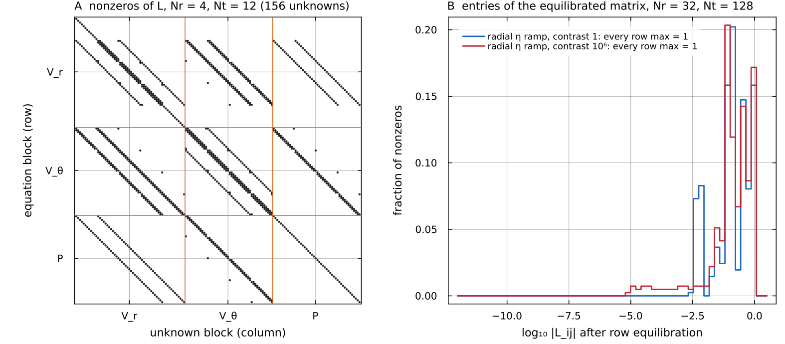
Left: the nonzeros of the matrix assemble_stokes returns for a $4\times 12$ annulus (156 unknowns), ordered $V_r$, $V_{\theta }$, $P$; the bands run parallel to the diagonal because $\theta$ varies fastest, and the short off-band runs are the periodic wrap. Right: the magnitudes of all entries after row equilibration on a $32\times 128$ annulus, for a uniform viscosity and for a radial viscosity ramp of contrast ${10}^6$. Every row has a largest entry of exactly 1 in both cases, so a contrast of ${10}^6$ in $\eta$ stretches the spread of the remaining entries by only a few decades. Script: docs/scripts/fig_numerics_discretization_sections.jl.

The viscous operator is ∇·(2η ε̇)

With cfg.useDeviatoricStress = true (the default) the viscous block is factored in _viscous_block_deviatoric:

$$L_{\text{visc}}=RS,S:(V_r,V_{\theta })\mapsto \tau =2\eta \dot{\epsilon },R:\tau \mapsto \text{momentum rows}.$$

Here $S$ is the discrete constitutive law, the only place viscosity appears, and $R$ is the discrete divergence. The strain-rate components are

$$\begin{array}{rl}{\dot{\epsilon }}_{rr}& ={\partial }_r{V}_r,\\ {\dot{\epsilon }}_{\theta \theta }& =\frac{1}{r}{\partial }_{\theta }{V}_{\theta }+\frac{V_r}{r},\\ {\dot{\epsilon }}_{\phi \phi }& =\frac{V_r}{r}(m=2\text{ only, the second hoop strain}),\\ {\dot{\epsilon }}_{r\theta }& =\frac{1}{2}[r{\partial }_r(V_{\theta }/r)+\frac{1}{r}{\partial }_{\theta }{V}_r],\end{array}$$

and the momentum rows are

$$\begin{array}{rl}r:& \frac{1}{r^m}{\partial }_r\left(r^m{\tau }_{rr}\right)+\frac{1}{r}{\partial }_{\theta }{\tau }_{r\theta }-\frac{{\tau }_{\theta \theta }}{r}-(m-1)\frac{{\tau }_{\phi \phi }}{r}-{\partial }_{r}P+b=0,\\ \theta :& \frac{1}{r^{m+1}}{\partial }_r\left(r^{m+1}{\tau }_{r\theta }\right)+\frac{1}{r}{\partial }_{\theta }{\tau }_{\theta \theta }-\frac{1}{r}{\partial }_{\theta }P=0.\end{array}$$

Because the operator is built as a product, $\mathrm{\nabla }\cdot (2\eta \dot{\epsilon })$ holds by construction and no viscosity-gradient term can be dropped by hand. ${\tau }_{rr}$, ${\tau }_{\theta \theta }$, ${\tau }_{\phi \phi }$ sit at cell centres; ${\tau }_{r\theta }$ sits on interior radial faces, where the viscosity is the arithmetic mean of the four surrounding cells. The trace of $\dot{\epsilon }$ is the discrete divergence for the matching $m$, so $\tau$ is trace-free on a discretely divergence-free solution.

For incompressible flow $\mathrm{\nabla }\cdot (2\eta \dot{\epsilon })=\eta {\mathrm{\nabla }}^2\mathbf{V}+2(\mathrm{\nabla }\eta )\cdot \dot{\epsilon }$, so the factored form carries the viscosity-gradient term automatically. Setting useDeviatoricStress = false selects the form $\eta {\mathrm{\nabla }}^2\mathbf{V}$, which equals Stokes only where $\eta$ is constant.

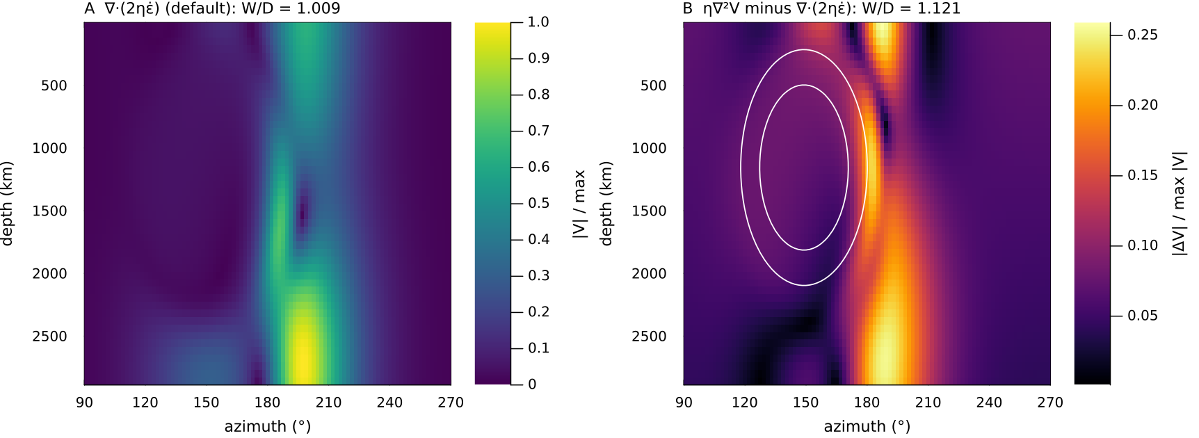
A hot blob beside a stiff inclusion (viscosity raised 1000 times, white contours at 10 and 100 times the background) in a $48\times 192$ spherical annulus, solved with assemble_stokes twice. Left: the speed from the default factored operator $RS$, for which work over dissipation is 1.009. Right: the difference to the $\eta {\mathrm{\nabla }}^2\mathbf{V}$ form (useDeviatoricStress = false), up to about a quarter of the peak speed, concentrated where the flow shears past the inclusion; that form returns $W/D$ = 1.12. A small grid chosen to illustrate the operator. Script: docs/scripts/fig_numerics_discretization_sections.jl.

How the operator is checked

Two properties hold exactly for any correct Stokes operator and are asserted in tests/test_annulus_operator.jl:

1. Work equals dissipation. For a Stokes solution under a body force $\mathbf{f}$,

$$W=\int \mathbf{f}\cdot \mathbf{V}dV=D=\int 2\eta \dot{\epsilon }:\dot{\epsilon }dV,$$

so $W/D=1$ at any viscosity field. Measured on a fixed analytic load:

Viscosity contrast	$W/D$ at $N_r$ = 24 / 48 / 96
1	0.995 / 0.999 / 1.000
10	0.996 / 0.999 / 1.000
${10}^3$	1.002 / 1.001 / 1.001
${10}^6$	1.019 / 1.006 / 1.003

2. Rigid rotation is a null mode. $\dot{\epsilon }\equiv 0$ for rigid rotation in every geometry. The deviatoric operator annihilates it to round-off in the spherical annulus as well ($1.5\times {10}^{-16}$, $1.4\times {10}^{-16}$, $2.3\times {10}^{-16}$ at $N_r$ = 12, 24, 48).

Rigid rotation alone cannot detect a missing $(\mathrm{\nabla }\eta )\cdot \dot{\epsilon }$ term, because that term vanishes on a strain-free field. The work-dissipation identity at variable viscosity is the check that does.

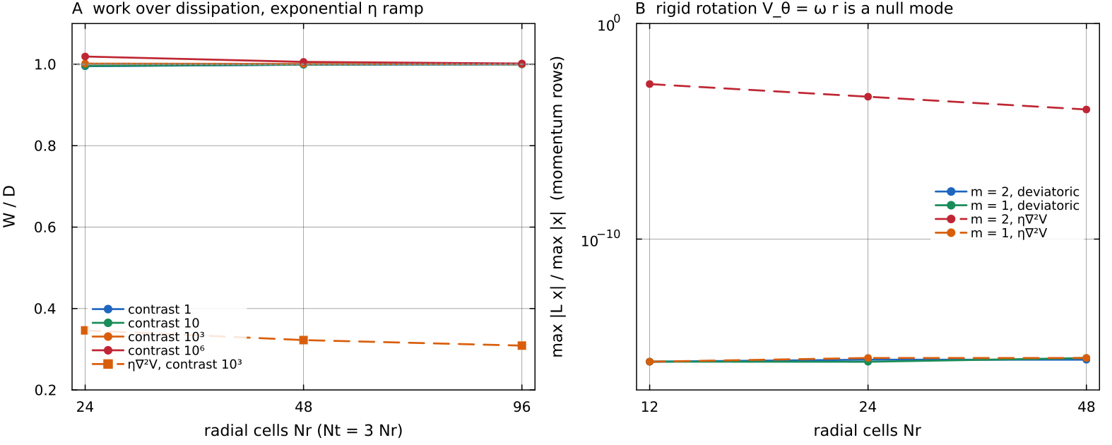
Both checks recomputed with the assembled operator. Left: $W/D$ for the load $\sin (\pi z/D)\cos 3\theta$ on an exponential viscosity ramp at $N_r$ = 24, 48, 96 ($N_t=3N_r$): the deviatoric operator approaches 1 at every contrast, while the $\eta {\mathrm{\nabla }}^2\mathbf{V}$ form stays near 0.31 to 0.35 at contrast ${10}^3$ and does not improve. The load is not the one of the table above, so the digits differ slightly. Right: the assembled matrix applied to the rigid rotation $V_{\theta }=\omega r$. The deviatoric operator returns round-off in both geometries; the $\eta {\mathrm{\nabla }}^2\mathbf{V}$ form leaves a first-order residual in the spherical annulus and none in the cylinder. Script: docs/scripts/fig_numerics_discretization_sections.jl.

Continuity, pressure and boundary conditions

The continuity row at each cell is

$$\frac{1}{r^m}\frac{r_{F,i+1}^m{V}_{r,i+1}-r_{F,i}^m{V}_{r,i}}{\mathrm{\Delta }{r}_i}+\frac{1}{r}\frac{V_{\theta ,j+1}-V_{\theta ,j}}{\mathrm{\Delta }\theta }=0.$$

cfg.pPen adds a pressure penalty to this row and is 0 by default. The staggered grid is inf-sup stable and needs no stabilisation; with no penalty the direct solvers return round-off divergence everywhere.

• Walls. $V_r=0$ at $R_{\text{in}}$ and $R_{\text{out}}$. Free slip is zero shear traction, ${\tau }_{r\theta }=0$, imposed by dropping the wall shear flux.

• Pressure null space. One pressure DOF near the domain centre is pinned. All 2-D solvers now pass point_pin=true (a single identity row). The older dense "mean pressure = 0" row is still available for point_pin=false; it replaces a continuity row, couples every pressure unknown, and is unusable by a local multigrid smoother.

• Rotation null space. One $V_{\theta }$ DOF is pinned in the assembly. After every 2-D solve main_SphCon.jl then removes the net rotation, the rigid rotation $\omega r$ that makes $\int \rho r{V}_{\theta }{r}^{m}drd\theta$ vanish (_net_rotation_rate, gated by cfg.removeNetRotation, default true). This projection has no effect in 3-D and the code warns if it is requested there.

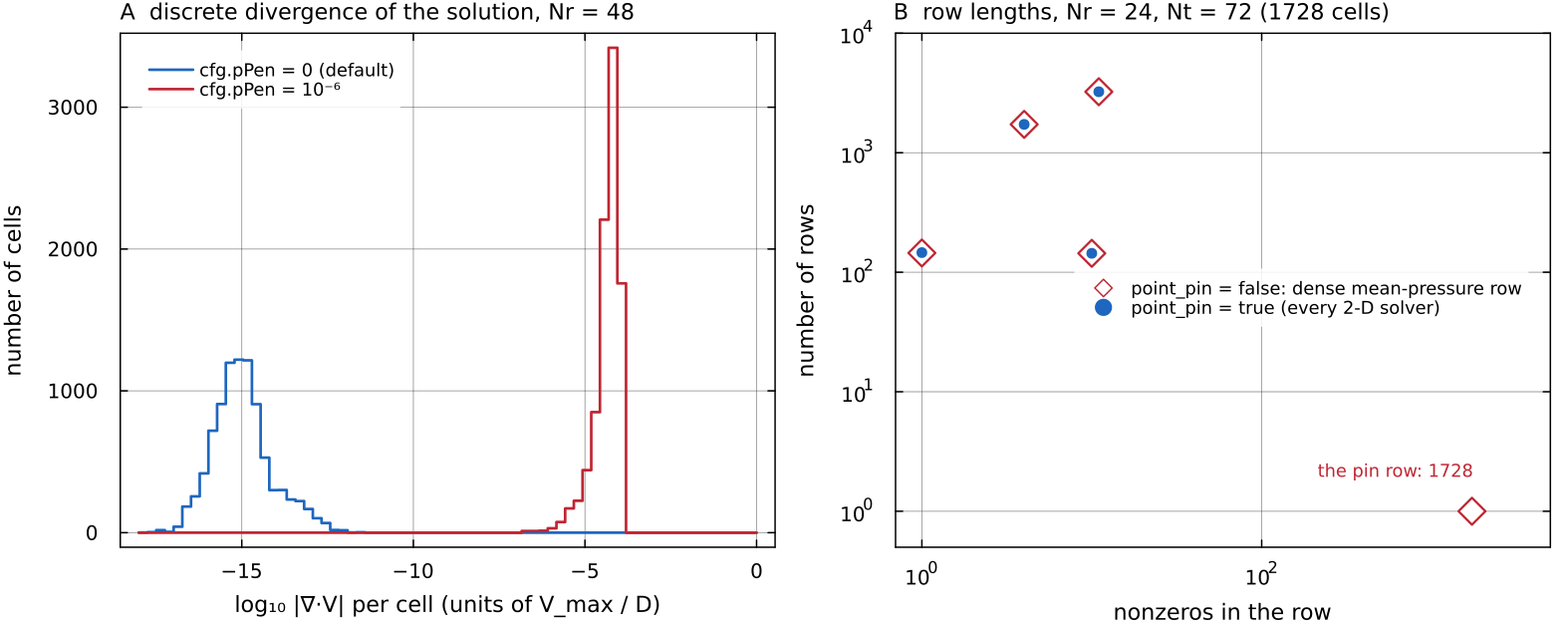
Left: the discrete divergence of each cell (the continuity row above, in units of $V_{\text{max}}/D$) for one solve on a $48\times 192$ annulus with a viscosity contrast of ${10}^3$; the pinned cell is excluded. With pPen = 0 the divergence is round-off, ${10}^{-15}$; a penalty of ${10}^{-6}$ raises it to about ${10}^{-4}$ in every cell. Right: the number of nonzeros per row for the two pressure pins on a $24\times 72$ annulus. The dense mean-pressure row couples all 1728 pressure unknowns; with point_pin = true the longest row has 11 entries and the rows of length 1 are the wall and pin identities. Script: docs/scripts/fig_numerics_discretization_sections.jl.

Radial grid stretching

_amr_radial_grid in utils/setup_grid.jl places the $N_r+1$ radial faces with a double-sided tanh map of a uniform parameter $\xi \in [0,1]$:

$$\zeta (\xi )=\frac{1}{2}[1+\frac{\tanh (\beta (\xi -\frac{1}{2}))}{\tanh (\beta /2)}],r_F=R_{\text{in}}+\zeta (\xi )D,$$

with $\beta$ = cfg.amrStretchFactor (default 0, uniform). Cells are smallest at both boundaries and largest at mid-depth; the source quotes $\beta =2$ as about 2.3:1 between boundary and interior cells. Cell centres are face midpoints. The grid stores

Field	Size	Meaning
grid.rF	$N_r+1$	face radii
grid.r	$N_r$	cell-centre radii
grid.drVec	$N_r$	cell widths $\mathrm{\Delta }{r}_i$
grid.drFVec	$N_r+1$	centre-to-centre spacing at each face, half a cell at the walls
grid.dr	scalar	the minimum cell width (used by the CFL limit)

The 2-D Stokes, diffusion, advection and marker routines all use drVec and drFVec. In 3-D the same radial map is used, and the tangential axes can be stretched in the same way through cfg.amrStretchTheta and cfg.amrStretchPhi (_amr_angular_grid).

On a stretched grid grid.dr is minimum(drVec), so a new radial derivative should use the local widths drVec or drFVec, and radial_cell_index (or searchsortedfirst on grid.r / grid.rF) to locate a radius.

The 2-D lateral spacing is uniform: MutableGrid2D.dth is a scalar and there is no lateral refinement in 2-D.

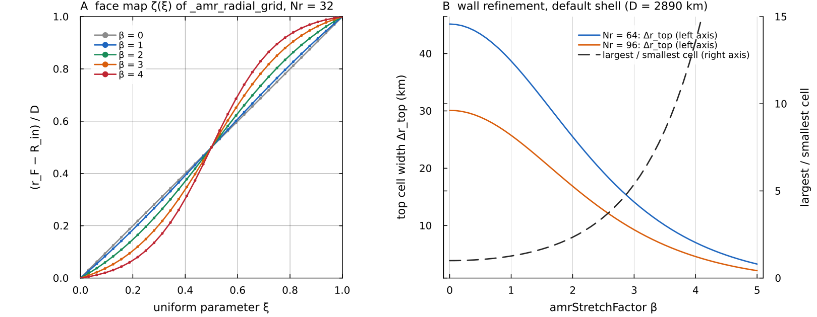
Left: the face positions $\zeta (\xi )$ that _amr_radial_grid returns for $N_r=32$ and $\beta$ = 0 to 4; the map is symmetric about mid-depth, so both walls are refined equally. Right: the width of the top cell of the default shell at $N_r$ = 64 and 96, and the ratio of the largest to the smallest cell (independent of $N_r$ at fixed $\beta$): $\beta =2$ gives about 2.3:1 and $\beta =3$ about 5.4:1, with a top cell of 9.3 km at $N_r=96$. Script: docs/scripts/fig_numerics_discretization_sections.jl.

The 3-D operator

assemble_stokes_3d integrates every row over its control volume so that the pressure-gradient block equals minus the transpose of the divergence block, $G=-B^{\mathsf{T}}$, at the matrix-entry level. This symmetry is what the multigrid smoother relies on; verify_g_minus_bt in the same file checks it on an assembled matrix. Measured on an $8\times 8\times 24$ Yin patch, excluding the pressure-pin and Dirichlet wall rows, $\parallel G+B^{\mathsf{T}}{\parallel }_{\mathrm{\infty }}=0$ exactly. No row equilibration is applied in 3-D, for the same reason.

• Layout. $V_r$ on radial faces $(N_r+1)\times N_{\theta }\times N_{\phi }$, $V_{\theta }$ on colatitude faces $N_r\times (N_{\theta }+1)\times N_{\phi }$, $V_{\phi }$ and $P$ at $N_r\times N_{\theta }\times N_{\phi }$, with $V_{\phi }[k]$ on the right face of cell $k$.

• Full stress. cfg.useCurvatureTerms = true (default) assembles the divergence of the full deviatoric stress with all six spherical strain components. The false branch is the componentwise scalar Laplacian. Measured on the two branches at $N_r$ = 8 / 12 / 16: rigid-rotation residual $2.0\times {10}^{-16}$ / $2.5\times {10}^{-16}$ / $2.5\times {10}^{-16}$ (true) against $9.8\times {10}^{-4}$ / $6.6\times {10}^{-4}$ / $4.5\times {10}^{-4}$ (false), and $W/D$ = 1.004 / 0.997 / 0.997 against 0.559 / 0.724 / 0.813.

• Variable viscosity. With a radial viscosity ramp on a Yin-Yang chunk, $W/D$ at $N_r$ = 8 / 12 / 16 is 0.9961 / 1.0026 / 1.0029 at contrast 1 and 0.9812 / 0.9813 / 0.9841 at ${10}^6$, improving under refinement at every contrast (tests/test_stokes_3d_variable_eta.jl).

• Face viscosities. With cfg.useGeometricEta = true (default) viscosities at velocity faces and edges are geometric means, $\sqrt{ab}$ for two cells and $(abcd{)}^{1/4}$ for four, following Tackley (2008, §3.2), who advises against arithmetic interpolation at large contrast. This applies to the 3-D assembly; the 2-D deviatoric ${\tau }_{r\theta }$ uses the arithmetic four-cell mean.

• $\phi$ edges. Each Yin-Yang patch is a non-periodic rectangle in $(\theta ,\phi )$; the viscous stencil is guarded at $k=1$ and $k=N_{\phi }$, and the walls take values from the other patch through the Schwarz iteration.

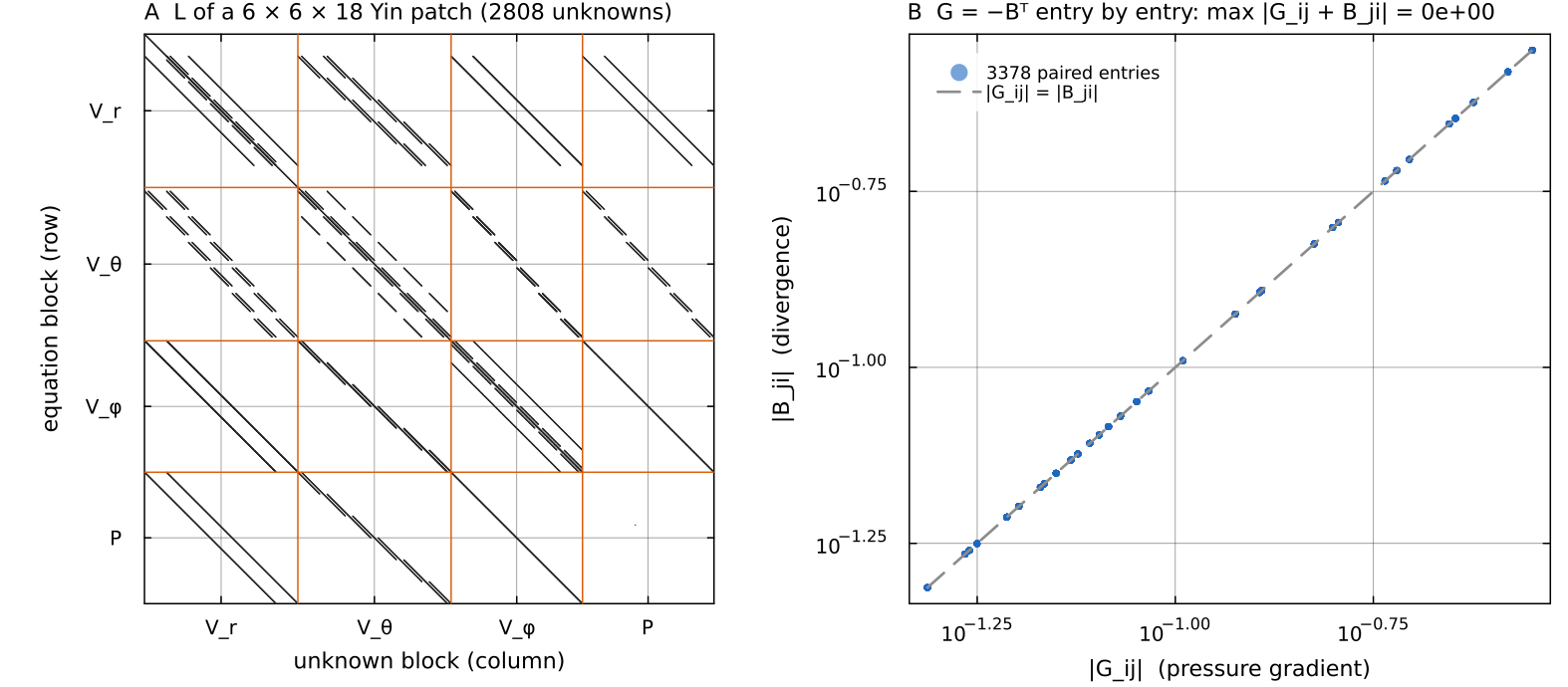
Left: the nonzeros of the matrix assemble_stokes_3d returns for a $6\times 6\times 18$ Yin patch (2808 unknowns), in the blocks $V_r$, $V_{\theta }$, $V_{\phi }$, $P$. Right: every entry of the pressure-gradient block $G$ against its transposed partner in the divergence block $B$ (from verify_g_minus_bt); all 3378 pairs agree to the last bit, $max|G_{ij}+B_{ji}|=0$. Only the assembly is needed, no 3-D solve. Script: docs/scripts/fig_numerics_discretization_sections.jl.

Where in the code

Topic	File	Function
Radial exponent $m$	utils/geometry.jl	geometry_exponent
2-D grid and stretching	utils/setup_grid.jl	_setup_grid_2d, _amr_radial_grid
2-D Stokes assembly	solvers/stokes_assembly.jl	assemble_stokes, _viscous_block_deviatoric, unpack_stokes
3-D Stokes assembly	solvers/stokes_assembly_3d.jl	assemble_stokes_3d, unpack_stokes_3d, verify_g_minus_bt
Net-rotation removal	main_SphCon.jl	_net_rotation_rate
Operator tests	tests/	test_annulus_operator.jl, test_spherical_operator_nullmode.jl, test_stokes_3d_variable_eta.jl, test_energy_consistency.jl