Heat sources and thermal boundaries

This page covers what heats and cools the mantle in the energy equation, and the temperature conditions at its two walls. Diffusion and sources are solved together by diffuse_temperature (solvers/diffuse_temperature.jl) after the temperature has been advected: by the markers in 2-D by default; in 3-D the Yin patch temperature is carried by the markers as in 2-D (cfg.temperatureOnGrid is ignored in 3-D), and the Yang patch temperature is advected on the grid with the first-order advect_temperature_3d_upwind!, whatever cfg.tempAdvectionScheme says. The time discretisation is Crank-Nicolson (cfg.useImplicitTemp = true, cfg.implicitTheta = 0.5; $\theta =1$ is backward Euler, false is explicit Euler).

The right-hand side the solver adds to the conduction term is

$$S=\frac{H(\mathbf{x},t)}{c_p}+\frac{Q(\mathbf{x},t)}{{\rho }_{\text{ref}}(r)c_p}[{\text{K s}}^{-1}],$$

with $H$ the mass-specific heating (W kg${}^{-1}$) and $Q$ the volumetric sources (W m${}^{-3}$). $c_p=1250$ J kg${}^{-1}$ K${}^{-1}$ everywhere. In 2-D and 3-D, ${\rho }_{\text{ref}}$ is the local reference density under ALA and TALA and ${\rho }_0$ under Boussinesq, the one profile reference_density (physics/compressibility.jl) that compressibility also returns.

Physical background

Where a planet's heat comes from

A rocky planet is a heat engine that is slowly running down. It formed hot, from the energy of accretion and of core formation, and it has been losing that heat through its surface ever since. At the same time the decay of long-lived radioactive isotopes of uranium, thorium and potassium keeps producing heat inside the silicate mantle and crust. The mantle therefore receives heat in three ways. It is heated from within by radioactive decay, from below through the core-mantle boundary (CMB) by a core that is itself cooling, and from its own store of sensible heat, which it gives up as it cools (secular cooling). It loses heat through the surface, where conduction across the cold outer boundary layer delivers it to the atmosphere or ocean.

For the Earth the sizes of these terms are constrained by observation. The surface heat flow is $47\pm 2$ TW (Davies & Davies 2010). The bulk silicate Earth composition of McDonough & Sun (1995), with 20.3 ppb U, 79.5 ppb Th and 240 ppm K, gives about $4.9\times {10}^{-12}$ W kg${}^{-1}$ with the specific heat productions MILEVA uses, or roughly 20 TW over the $4.0\times {10}^{24}$ kg of mantle and crust. A large part of that sits in the continental crust, so the convecting mantle produces less. The heat flowing out of the core is estimated at 5 to 15 TW (Lay et al. 2008). The ratio of internal heat production to surface heat loss is the Urey ratio. Korenaga (2008) estimates it at about 0.35 for the bulk Earth and about 0.2 for the convecting mantle alone, so most of the present heat loss is paid for by secular cooling and by the core rather than by radioactivity.

These numbers are why the source terms on this page decide the long-term behaviour of a model. A run whose heat production exceeds what its lid can conduct away warms, and one that produces less cools. The balance shifts with time, because radioactive heating decays and the core cools, and the thermal history of a planet is the slow approach of these terms towards each other.

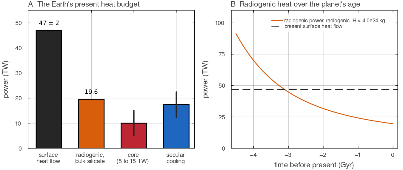
A: surface heat flow (Davies & Davies 2010), the radiogenic power of the bulk silicate Earth computed by radiogenic_H with the McDonough & Sun (1995) concentrations over $4.0\times {10}^{24}$ kg, 19.6 TW, the 5 to 15 TW core heat flow of Lay et al. (2008), and secular cooling as the remainder. B: the same radiogenic power back in time; it exceeded the present surface heat flow before about 3.1 Gyr ago. Script: docs/scripts/fig_heat_sources_sections.jl.

Radioactive decay

Each radioactive isotope decays exponentially with its own half-life. Its heat production per kilogram of rock is its concentration times the power released per kilogram of the isotope. Four isotopes matter over the age of the Solar System.

isotope	half-life (Gyr)	share of the present heat production with MILEVA's default concentrations
U-238 and U-235	4.468 and 0.704	41 %
Th-232	14.05	42 %
K-40	1.277	17 %

The half-lives are those tabulated in utils/radiogenic.jl, after Turcotte & Schubert (2002, Table 4.2), and the shares follow from those values and the default concentrations. Because U-235 and K-40 decay quickly, heat production was much larger in the past. With the default concentrations the four-isotope sum 4.5 Gyr before the time at which the concentrations hold is about 4.7 times its value at that time. A 4.5 Gyr thermal history therefore starts with a strongly heated mantle and ends with a weakly heated one. The single-rate law in MILEVA replaces the isotope mix by one effective half-life. A half-life of 2.43 Gyr, as in the pipeline example below, follows the overall decline over a planet's lifetime without resolving the change in isotope mix. Aluminium-26, with a half-life of 0.717 Myr, mattered only in the first few million years of the Solar System and is relevant only to models of planetesimals and early bodies.

Uranium, thorium and potassium are incompatible elements. Their large ions do not fit well into the crystal lattices of mantle minerals, so when rock partially melts they enter the melt preferentially. The partition coefficient $D$, the ratio of the concentration in the solid to that in the melt, is much smaller than one (the pipeline example uses $D=0.001$). Melting therefore strips the heat sources out of the residue and carries them upwards into the crust. The Earth's bulk continental crust holds about 1.3 ppm U (Rudnick & Gao 2003), some sixty times the primitive-mantle value above. This is the physical reason for the composition factors in MILEVA. Crust and enriched material heat more strongly than average mantle, and melt-depleted residue heats more weakly.

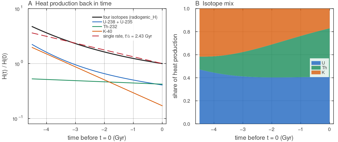
A: radiogenic_H with the default concentrations (21 ppb U, 80 ppb Th, 250 ppm K), in total and per chain, normalised by the total at $t=0$, and the single-rate law of _radiogenic_H0 with a half-life of 2.43 Gyr; the total is 4.7 times higher 4.5 Gyr earlier. B: the share of uranium, thorium and potassium in the total; uranium and potassium carry most of it early, thorium more than 40 per cent today. Script: docs/scripts/fig_heat_sources_sections.jl.

Internal heating and basal heating

Where the heat enters changes the character of convection (Schubert, Turcotte & Olson 2001). A layer heated from below has two thermal boundary layers of comparable strength. Hot plumes rise from the bottom boundary layer and cold sheets sink from the top one. A layer heated from within has no hot boundary layer at its base. Its interior is warm and nearly uniform, and the flow is driven mainly by cold downwellings from the top, with broad, slow return flow. Real mantles are heated in both ways, and the proportion of basal to internal heating sets how strong plumes are compared with downwellings. Two consequences follow for a model. The mean interior temperature depends on the internal heating rate, not only on the wall temperatures. And the core heat flow is not fixed in advance. It is whatever the bottom boundary layer conducts, which depends on how hot the lower mantle is.

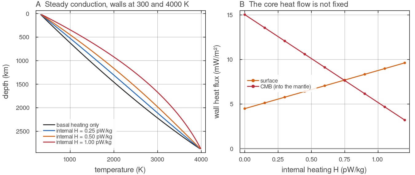
Steady states of diffuse_temperature (backward Euler, conduction only, no flow) in the default shell with the walls at 300 and 4000 K, and the wall fluxes from boundary_power. A conducting shell carries little heat, so the heating rates are far below planetary values; the picture shows the mechanism. A: internal heating bends the profile and warms the interior. B: as the interior warms, the heat flowing in from the core falls, from 15 mW m${}^{-2}$ with basal heating only to 3 mW m${}^{-2}$ at 1.2 pW kg${}^{-1}$, while the surface flux rises. Script: docs/scripts/fig_heat_sources_sections.jl.

Adiabatic compression and viscous dissipation

Mantle rock is slightly compressible. A parcel that sinks is compressed by the increasing pressure and warms, and one that rises expands and cools. Without any heat exchange this gives the adiabatic temperature gradient

$${\left(\frac{dT}{dz}\right)}_{\text{ad}}=\frac{\alpha gT}{c_p},$$

with $\alpha$ the thermal expansivity, $g$ gravity, $T$ the absolute temperature, $c_p$ the specific heat and $z$ depth. With $\alpha =3\times {10}^{-5}$ K${}^{-1}$, $g=9.81$ m s${}^{-2}$, $T=1600$ K and $c_p=1250$ J kg${}^{-1}$ K${}^{-1}$ this is about 0.4 K km${}^{-1}$. In the energy equation the same physics appears as the volumetric source $-\rho \alpha gT{V}_r$. It is negative where material moves up ($V_r>0$) and positive where it moves down. Its strength relative to the other terms is measured by the dissipation number $Di=\alpha gD/c_p$ (see Governing equations).

Deformation of a viscous material converts mechanical work into heat at the rate ${\tau }_{ij}{\dot{\epsilon }}_{ij}$. For an incompressible viscous fluid this is $2\eta {\dot{\epsilon }}_{ij}{\dot{\epsilon }}_{ij}$, which equals $4\eta {\dot{\epsilon }}_{II}^2$ with ${\dot{\epsilon }}_{II}=\sqrt{\frac{1}{2}{\dot{\epsilon }}_{ij}{\dot{\epsilon }}_{ij}}$. The two terms are linked. In a statistically steady convecting layer the work done by buoyancy forces is dissipated as heat, and the volume integral of the viscous dissipation equals the volume integral of the adiabatic cooling. Carried together, neither changes the total heat budget, while carrying only one creates or destroys energy (Leng & Zhong 2008). Locally they do not cancel. Dissipation concentrates where the strain rate is high, in boundary layers and shear zones, while adiabatic heating and cooling follow the vertical flow. This is why MILEVA switches the two terms on and off together.

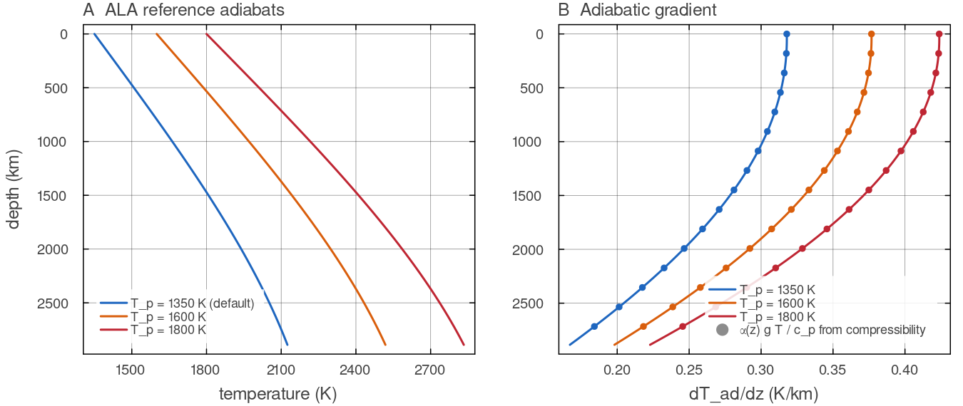
A: adiabat_temperature on the default shell (Earth-sized, $g$ = 9.81 m s${}^{-2}$, $\alpha$ falling from $3\times {10}^{-5}$ at the surface to ${10}^{-5}$ K${}^{-1}$ at the CMB). B: the gradient of each adiabat (lines) and $\alpha (z)gT/c_p$ evaluated with the expansivity that compressibility returns (dots); they agree, at 0.32 to 0.42 K km${}^{-1}$ near the surface, falling with depth as $\alpha$ decreases. Script: docs/scripts/fig_heat_sources_sections.jl.

Latent heat

Melting absorbs heat and freezing releases it. The solid-state phase transitions of the mantle, olivine to wadsleyite near 410 km and ringwoodite to bridgmanite and ferropericlase near 660 km, also release or absorb latent heat as material crosses them. That heat changes the temperature of material crossing a transition and so contributes to how strongly the transition helps or hinders flow (Christensen & Yuen 1985). Rising mantle that melts is cooled by the heat of fusion, and magma that freezes at shallow depth heats its surroundings. The Phase changes and Melting pages describe these terms in full.

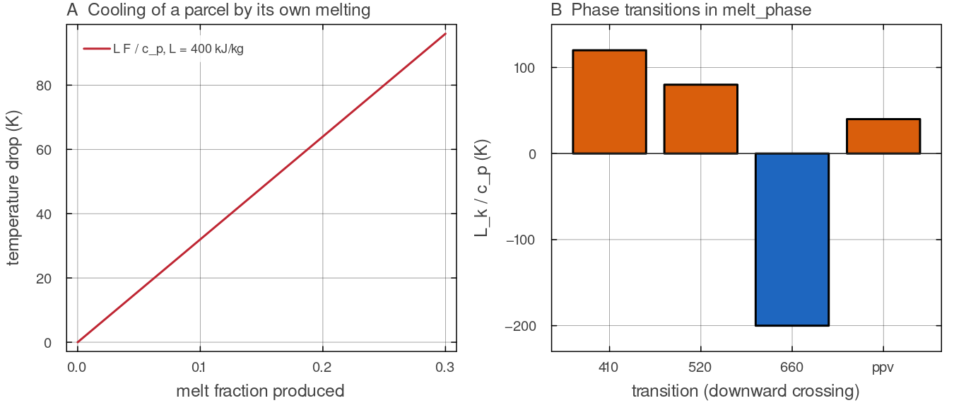
A: the cooling $LF/c_p$ of a parcel that melts a fraction $F$, with cfg.latentHeatMelt = 400 kJ kg${}^{-1}$ and $c_p$ = 1250 J kg${}^{-1}$ K${}^{-1}$. B: $L_k/c_p$ for the transitions melt_phase carries, positive for the exothermic transitions that warm material crossing them downward and negative for the endothermic one near 660 km. Script: docs/scripts/fig_heat_sources_sections.jl.

The core as a heat reservoir

The core is a large reservoir of heat that the mantle draws on through its base. To first order it is a well-mixed liquid whose temperature changes only as fast as the mantle extracts heat from it. Its heat capacity is ${\rho }_c{c}_c{V}_{\text{core}}$. For an Earth-sized core with MILEVA's default values (${\rho }_c=12000$ kg m${}^{-3}$, $c_c=800$ J kg${}^{-1}$ K${}^{-1}$, $R_{\text{in}}=3481$ km) this is about $1.7\times {10}^{27}$ J K${}^{-1}$, and a CMB heat flow of 10 TW then cools the core by about 190 K Gyr${}^{-1}$. For comparison, the density of the Earth's core in the Preliminary Reference Earth Model rises from about 9900 kg m${}^{-3}$ at the CMB to about 13 100 kg m${}^{-3}$ at the centre (Dziewonski & Anderson 1981). A real core has further energy sources. Growth of a solid inner core releases latent heat and gravitational energy, as light elements expelled at the inner-core boundary rise through the liquid, and these slow the cooling for a given heat flow (Stevenson, Spohn & Schubert 1983; Nimmo 2015). The CMB heat flow also matters beyond the mantle, because it decides whether the core convects vigorously enough to sustain a magnetic field (Stevenson, Spohn & Schubert 1983).

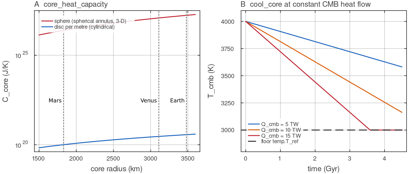
A: core_heat_capacity with the default core density and specific heat, for the spherical annulus and 3-D shell (a sphere of radius $R_{\text{in}}$) and for the cylindrical annulus (a disc per metre of length), with the core radii of Mars, Venus and the Earth marked. B: repeated cool_core calls for the default Earth core at constant CMB heat flow; 10 TW lowers $T_{\text{cmb}}$ by about 190 K Gyr${}^{-1}$, and at 15 TW the core reaches the floor temp.T_ref after 3.6 Gyr. Script: docs/scripts/fig_heat_sources_sections.jl.

Boundary layers and wall conditions

Heat crosses the top and bottom of a convecting mantle by conduction through thin thermal boundary layers, because the flow normal to a wall vanishes there. The heat flux through a wall is $q=-k\partial T/\partial r$, with $k$ the thermal conductivity, and a boundary layer of thickness $\delta$ across which the temperature changes by $\mathrm{\Delta }{T}_{\delta }$ carries $q\approx k\mathrm{\Delta }{T}_{\delta }/\delta$. The Nusselt number compares this flux with the flux that pure conduction across the whole layer would carry (see Governing equations). In a model the walls are usually held at fixed temperatures. At the surface this stands in for an atmosphere or ocean whose temperature changes little over geological time. At the CMB it stands in for a core whose temperature changes slowly, and MILEVA either holds it fixed or evolves it by the core energy balance described below.

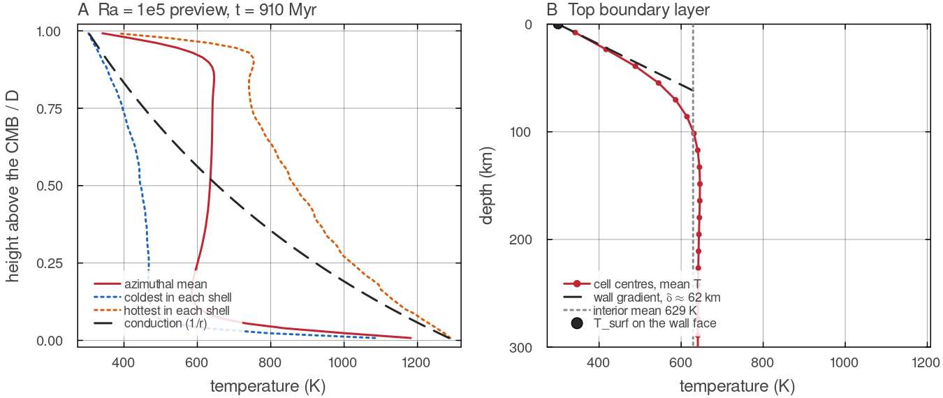
The last frame (910 Myr, 3000 steps) of the short Ra = ${10}^5$ preview of examples/annulus_convection_2d.jl (Hernlund & Tackley 2008 shell, walls at 300 and 1300 K, Nr = 64), read from its VTK output; it is a preview, not a statistically steady state. A: the interior is nearly isothermal at 629 K and the temperature changes in thin layers at both walls, unlike the conduction profile. B: the top boundary layer cell by cell; the gradient between the wall face and the first cell centre, extrapolated to the interior temperature, gives a thickness of about 62 km. Script: docs/scripts/fig_heat_sources_sections.jl.

Typical values for the Earth and Venus

quantity	Earth	Venus	source
surface heat flow	$47\pm 2$ TW	not measured; inferred from models and lithospheric structure	Davies & Davies (2010); Nimmo & McKenzie (1998)
radiogenic heat production of the bulk silicate planet, present	about $5\times {10}^{-12}$ W kg${}^{-1}$	usually assumed similar to the Earth's	McDonough & Sun (1995), with the specific heats above
Urey ratio	about 0.35 bulk, 0.2 convective	unknown	Korenaga (2008)
CMB heat flow	5 to 15 TW	unknown	Lay et al. (2008)
surface temperature	MILEVA default 300 K	about 735 K	Seiff et al. (1985)
upper-mantle adiabatic gradient	about 0.4 K km${}^{-1}$	similar	the formula above

Venus is close to the Earth in size and bulk composition, so its heat production is usually taken to be similar. Its surface is a single lid, with no plate tectonics today (Nimmo & McKenzie 1998). A single lid conducts heat out less efficiently than mobile plates, so for the same heat production the interior of Venus can retain more of its heat. The balance between radiogenic heating, core heat and surface loss is therefore a first-order question for Venus models.

Source terms

Each step, the code works out how fast every cell would warm or cool if no heat were conducted away, and then lets conduction redistribute that heat. The radiogenic part starts from one planet-wide rate that decays with time and is then scaled cell by cell according to what the cell is made of. Under the compressible (ALA) equations two more terms appear. Rising material cools as it expands and sinking material warms as it is compressed, and flow warms the rock it deforms. At the bottom wall the core feeds heat through the CMB face, and in the parameterised mode the core cools by exactly the heat it hands over.

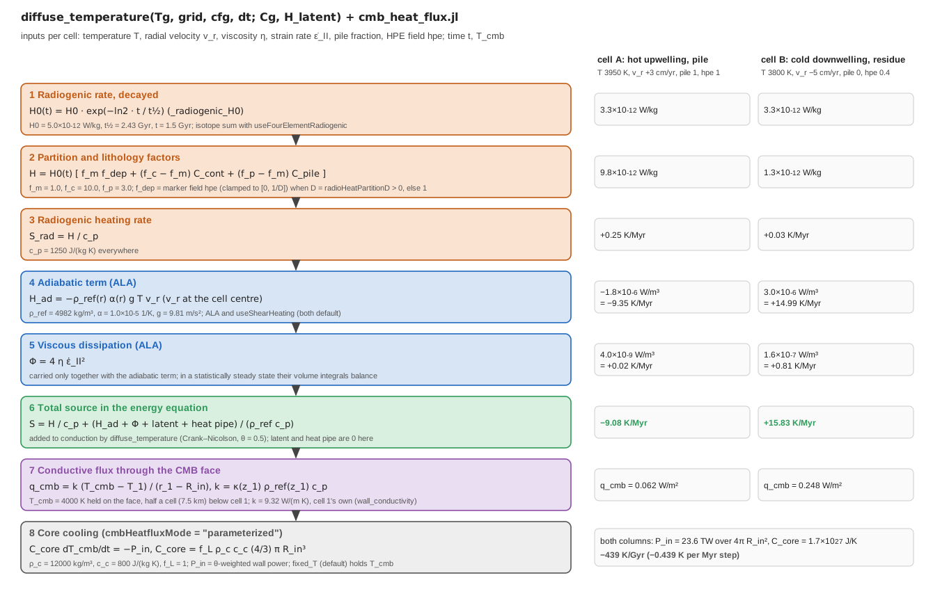
The two example cells sit in the bottom row of the default shell ($N_r=192$, 7.5 km above the CMB, $T_{\text{cmb}}=4000$ K), with single-rate radiogenic heating switched on ($t_{1/2}=2.43$ Gyr, read at $t=1.5$ Gyr), HPE partitioning ($D=0.001$) and the parameterised core. Cell A, a hot upwelling over a pile (3950 K, $+3$ cm yr${}^{-1}$), gains $+0.25$ K Myr${}^{-1}$ from radiogenic heat but loses $9.35$ K Myr${}^{-1}$ to adiabatic expansion, a net $-9.08$ K Myr${}^{-1}$; cell B, a cold downwelling carrying residue (3800 K, $-5$ cm yr${}^{-1}$, hpe 0.4), gains $+15.83$ K Myr${}^{-1}$, almost all of it from compression. The two columns draw $0.062$ and $0.248$ W m${}^{-2}$ from the core, which then cools at about 439 K Gyr${}^{-1}$. Script: docs/scripts/fig_heat_sources_pipeline.jl.

source	switch	form	where
radiogenic, single rate	cfg.useRadiogenicHeating	$H_0{2}^{-t/t_{1/2}}$ times lithology and partition factors	_radiogenic_H0, diffuse_temperature
radiogenic, four isotopes	cfg.useFourElementRadiogenic (with the above)	U-238, U-235, Th-232, K-40, Al-26 decay	radiogenic_H (utils/radiogenic.jl)
uniform internal heating	cfg.useInternalHeating	cfg.internalHeating_H (W kg${}^{-1}$), no decay, no composition weighting	diffuse_temperature
two-layer heating	temp.useLayeredHeating	temp.H_upper above mid-depth, temp.H_lower below	diffuse_temperature
latent heat of melting	cfg.useMeltingPhase	$-{\rho }_{0}LDF/Dt$ on the grid	melt_phase (physics/melt_phase.jl)
latent heat of phase transitions	cfg.useMeltingPhase and cfg.usePhaseLatentHeat	${\rho }_0{L}_{k}D{\mathrm{\Gamma }}_k/Dt$	melt_phase
magmatic heat transport	cfg.trackBasalt and cfg.useHeatPipe	heat pipe, see Melting	basalt_evolution!
adiabatic heating	ALA and cfg.useShearHeating	$-{\rho }_{\text{ref}}\alpha gT{V}_r$	compressibility, main_SphCon.jl
viscous dissipation	ALA and cfg.useShearHeating	$4\eta {\dot{\epsilon }}_{II}^2$	main_SphCon.jl

All terms add. The volumetric terms are collected into one field in main_SphCon.jl (the source assembly before the call to diffuse_temperature), and every logging interval the driver prints each one as the surface heat flux it would carry, in mW m${}^{-2}$, next to its cumulative effect on the mean temperature, so the energy equation can be read off the log.

Radiogenic heating

The single-rate law decays with half-life cfg.radioHeatingTau (years; 0 means constant) from cfg.radioHeatingH0 (default $5\times {10}^{-12}$ W kg${}^{-1}$) at $t=0$. With cfg.useFourElementRadiogenic = true the rate is instead

$$H(t)=\sum _i{c}_i{h}_i\exp (-\ln 2\frac{t}{t_{1/2,i}}),$$

from the concentrations cfg.radio_U_ppb (21), radio_Th_ppb (80), radio_K_ppm (250) and radio_Al26_kgkg (0), with the half-lives and specific heat productions tabulated in utils/radiogenic.jl (U split 99.28 / 0.72 % between U-238 and U-235, K-40 at 0.0117 % of K). Time runs forward from the concentrations given: $t=0$ is the moment those concentrations hold.

The local rate (2-D) is

$$H=H_0(t)[f_{\text{mantle}}{f}_{\text{dep}}+(f_{\text{cont}}-f_{\text{mantle}})C_{\text{cont}}+(f_{\text{pile}}-f_{\text{mantle}})C_{\text{pile}}],$$

with cfg.radioHeatMantleFactor (1), radioHeatContFactor (10) for painted crust and radioHeatPileFactor (3) for pile material. $f_{\text{dep}}$ is the heat-producing-element factor of melt depletion (_hpe_partition_factor): 1 when cfg.radioHeatPartitionD = 0 (default), otherwise the projected conserved marker field hpe that basalt_evolution! fractionates at extraction (see Melting). The 3-D solver applies $H_0(t)f_{\text{dep}}$ only, without the lithology factors.

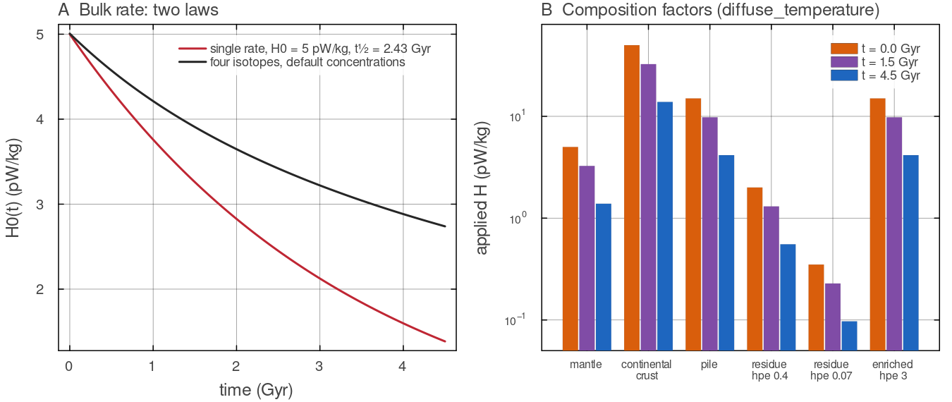
A: _radiogenic_H0 for the single-rate law ($H_0$ = 5 pW kg${}^{-1}$, $t_{1/2}$ = 2.43 Gyr) and for the four-isotope law with the default concentrations. B: the rate one explicit diffuse_temperature step applies to six columns of a uniform field (walls at the same temperature, so the change is the source alone), single-rate law with $D$ = 0.001: mantle 5, painted crust 50, pile 15, and residue with hpe 0.4 and 0.07 at 2 and 0.35 pW kg${}^{-1}$ at $t=0$, enriched material with hpe 3 at 15. Script: docs/scripts/fig_heat_sources_sections.jl.

Latent heat

The latent heat of melting on the grid, $-{\rho }_{0}LDF/Dt$, and of the solid-state transitions, ${\rho }_0{L}_{k}D{\mathrm{\Gamma }}_k/Dt$, are both returned by melt_phase when cfg.useMeltingPhase = true; the second needs cfg.usePhaseLatentHeat = true as well. The driver rescales them by $\mathrm{\Delta }{t}_{\text{prev}}/\mathrm{\Delta }t$ so that the energy applied over the step equals the energy booked. Their forms, the latent heats and the hand-off to the marker heat pipe are on the Phase changes page.

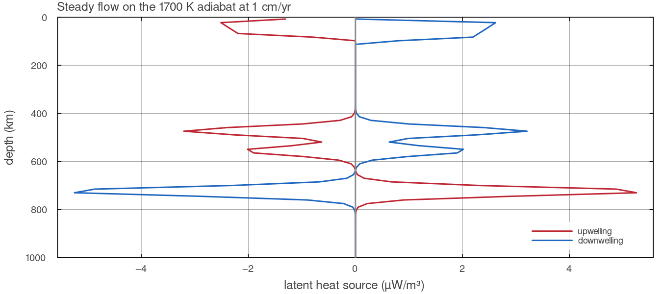
melt_phase with cfg.usePhaseLatentHeat = true on a column of the default shell (Nr = 192) on the 1700 K adiabat, with a uniform radial velocity of 1 cm yr${}^{-1}$ and no change in time, so the source is the advective part $v_r\partial F/\partial r$ and $v_r\partial {\mathrm{\Gamma }}_k/\partial r$ of the material derivatives. Upwelling material absorbs heat where it starts to melt near the surface and at the exothermic transitions, and releases it at the endothermic one; downwelling reverses every sign. Script: docs/scripts/fig_heat_sources_sections.jl.

Adiabatic heating and viscous dissipation

These are the two terms of order $Di$ in the compressible energy equation. They are carried together or not at all, under compressibilityMode = "ALA" and cfg.useShearHeating = true (both default). Their volume integrals balance in a statistically steady layer, so carrying one alone injects or drains the buoyancy work. TALA and Boussinesq carry neither.

In the code the adiabatic term is evaluated cell by cell as $-{\rho }_{\text{ref}}\alpha gT{V}_r$, with the prefactor ${\rho }_{\text{ref}}\alpha gT$ returned by compressibility (physics/compressibility.jl) from the advected temperature of the step, so it uses the full temperature and not only the reference adiabat, and with $V_r$ the mean of the radial velocities on the cell's lower and upper faces. The expansivity is the depth-dependent $\alpha (z)$ of the ALA reference state. The dissipation $4\eta {\dot{\epsilon }}_{II}^2$ is built in main_SphCon.jl from the viscosity and strain rate of the step and is also written to the VTK output.

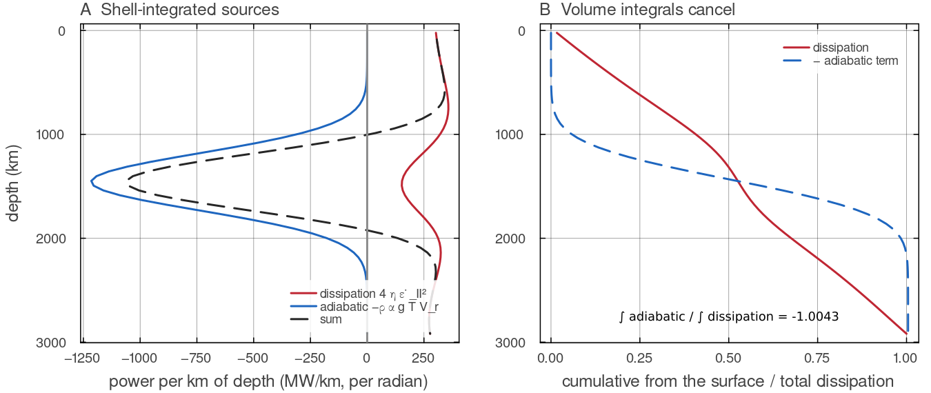
One Stokes solve (assemble_stokes, direct) on a Venus-sized spherical annulus (Nr = 64, Nt = 256, Boussinesq, isoviscous ${10}^{21}$ Pa s) driven by a +100 K blob of 300 km radius at mid-depth, with the dissipation $4\eta {\dot{\epsilon }}_{II}^2$ from compute_strain_rate and the adiabatic term $-{\rho }_0\alpha gT{V}_r$ for a 1600 K background. A: per shell the two terms differ greatly; the adiabatic term follows the vertical flow through the blob and the dissipation is spread over the whole cell of flow. B: their volume integrals cancel, the ratio being $-1.004$ at this resolution. Script: docs/scripts/fig_heat_sources_sections.jl.

Thermal boundary conditions

wall	condition
surface $r=R_{\text{out}}$	$T=T_{\text{surf}}$ = temp.T_surf (300 K default)
CMB $r=R_{\text{in}}$	$T=T_{\text{cmb}}$, the evolving grid.T_cmb (initially temp.T_cmb)
azimuth (2-D)	periodic
3-D Yin-Yang patch edges	Dirichlet values sampled from the other patch, cfg.nTSchwarz Schwarz sweeps per step

The Dirichlet value lives on the wall face, not in a cell. The first and last cells are ordinary flow cells. The wall temperature enters the conduction stencil through a half-cell ghost, so the wall flux is

$$q_{\text{wall}}=k\frac{T_{\text{bc}}-T_{\text{wall cell}}}{\mathrm{\Delta }r/2},k=\kappa {\rho }_{\text{ref}}{c}_p,$$

with $\kappa$ and ${\rho }_{\text{ref}}$ of the wall cell (wall_conductivity), and the grid advection schemes (utils/advect_temperature.jl) reflect the face value, $T_{\text{ghost}}=2T_{\text{bc}}-T_{\text{wall cell}}$. Inside the domain the operator uses the same conductivity: the flux through an interior face carries the mean of ${\rho }_{\text{ref}}\kappa c_p$ of the two cells that share it, and each cell divides its net flux by its own ${\rho }_{\text{ref}}{c}_p$ (conduction_coefficients), so the energy one cell loses through a face is the energy its neighbour gains. The wall value returned by wall_conductivity is the wall-face entry of the same coefficients, so there is one definition. The conductive reference of the Nusselt numbers (conductive_baseline_C) is the steady conduction profile of this same operator, with $r^{m}k\partial T/\partial r$ constant and $k={\rho }_{\text{ref}}{c}_p\kappa$, so $Nu=1$ on a conducting shell under ALA as under Boussinesq. No cell is overwritten. The same face flux is what the Nusselt numbers, the surface heat flow and the CMB heat flow report (compute_diagnostics, cmb_conductive_flux), so the discrete energy budget closes: tests/test_nusselt_conduction.jl checks $Nu=1$ on the solver's own conducting steady state and $N{u}_{\text{top}}=N{u}_{\text{bot}}$ to round-off, tests/test_energy_reference_state.jl checks the same under ALA with the pyrolite table on an Earth shell, together with $P_{\text{bot}}-P_{\text{top}}=dE/dt$ for one conduction step in 2-D and 3-D, and tests/test_conduction_conservation.jl checks that the radial conduction term is an exact flux difference.

In 3-D, temp.T_cmb_patches can add Gaussian hot or cold patches to the CMB temperature (cmb_temperature_field, config/TemperatureConditions.jl); the 2-D solver uses the uniform value.

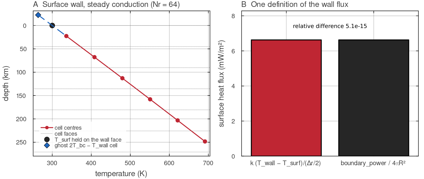
A steady conduction state of diffuse_temperature in the default shell (Nr = 64, 0.5 pW kg${}^{-1}$ internal heating). A: the six top cell centres, the faces, $T_{\text{surf}}$ held on the wall face and the ghost value $2T_{\text{bc}}-T_{\text{wall cell}}$ half a cell beyond it. B: the flux $k(T_{\text{wall cell}}-T_{\text{surf}})/(\mathrm{\Delta }r/2)$ with the conductivity of wall_conductivity, and the surface power of boundary_power divided by $4\pi R_{\text{out}}^2$; both give 6.627 mW m${}^{-2}$. Script: docs/scripts/fig_heat_sources_sections.jl.

Core-mantle boundary modes

cfg.cmbHeatfluxMode decides how $T_{\text{cmb}}$ evolves (physics/cmb_heat_flux.jl):

mode	behaviour
"fixed_T" (default)	constant $T_{\text{cmb}}$; with temp.cmb_cooling = true it falls linearly at temp.cmb_cooling_rate K Gyr${}^{-1}$
"fixed_flux"	$T_{\text{cmb}}$ is nudged each step (damping 0.1) so the mean conductive CMB flux tracks cfg.cmbHeatflux (W m${}^{-2}$)
"parameterized"	the core cools by the heat it delivers to the mantle

In the parameterised mode the core is a well-mixed sensible-heat reservoir with no inner core and no internal heating:

$$C_{\text{core}}\frac{d{T}_{\text{cmb}}}{dt}=-Q_{\text{cmb}},C_{\text{core}}=f_L{\rho }_c{c}_c{V}_{\text{core}},$$

with ${\rho }_c$ = cfg.coreDensity (12 000 kg m${}^{-3}$), $c_c$ = cfg.coreCp (800 J kg${}^{-1}$ K${}^{-1}$) and $f_L$ = cfg.coreLatentFactor (1; values above 1 are a crude stand-in for latent and gravitational energy). $V_{\text{core}}$ and the CMB area follow the mantle's geometry (core_heat_capacity, cmb_area): a sphere of radius $R_{\text{in}}$ behind $4\pi R_{\text{in}}^2$ for the spherical annulus and the 3-D shell, a disc behind $2\pi R_{\text{in}}$ per unit length for the cylindrical annulus. In 2-D the core is debited after the temperature step by exactly the energy the mantle took in through its base during that step (cool_core, using the solver's own $\theta$-weighted wall power), so core plus mantle conserves energy to round-off, under Boussinesq and ALA alike: the wall power uses the same conductivity as the diffusion operator (wall_conductivity, see the note on the CMB conductivity below). The 3-D path still debits at the start of the step.

temp.T_ref (default 3000 K) is a floor on an evolving $T_{\text{cmb}}$. It is a real temperature: a run in the potential-temperature frame, whose core sits lower, must lower it, and main_SphCon refuses to start a parameterised run whose initial $T_{\text{cmb}}$ is below the floor. In "fixed_flux" mode, and in "fixed_T" with temp.cmb_cooling = true, the same floor applies in cmb_heat_flux (physics/cmb_heat_flux.jl) but is not checked at start-up: a run with $T_{\text{cmb}}$ below temp.T_ref is lifted to the floor on its first update, so lower temp.T_ref for such runs.

Under ALA the conductivity at the CMB is $\kappa {\rho }_{\text{ref}}{c}_p$ of the first cell, the value the diffusion operator applies across the CMB face and with which that cell banks the energy. The reported $q_{\text{cmb}}$ (cmb_conductive_flux) and the wall power that debits the core (boundary_power) both read it from wall_conductivity, so the core loses exactly the energy the bottom cells gain; tests/test_energy_reference_state.jl checks this to round-off under ALA. Under Boussinesq it is the constant $\kappa {\rho }_0{c}_p$.

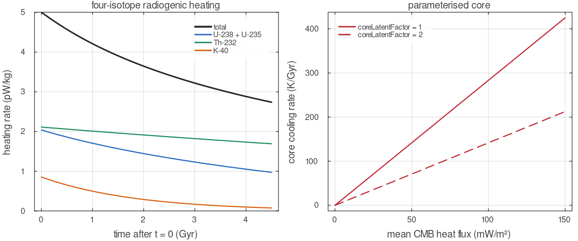
Left: radiogenic_H with the default concentrations, in total and per isotope chain. Right: the cooling rate of the parameterised core, $Q_{\text{cmb}}/C_{\text{core}}$, from core_heat_capacity and cmb_area for the default core, as a function of the mean CMB heat flux.

Initial temperature

temp.initial_profile selects the background (2-D marker initialisation, markers/init_markers.jl):

value	background
"adiabatic" (default)	the reference adiabat $T_{\text{ad}}(z)$ plus exponential boundary layers of thickness temp.tbl_top_thickness and temp.tbl_bottom_thickness. With the default thicknesses (both 0, config/TemperatureConditions.jl) the profile is a linear ramp from $T_{\text{cmb}}$ to $T_{\text{surf}}$; the adiabat with boundary layers is used only when a thickness is set
"conductive"	$T_{\text{surf}}+\mathrm{\Delta }T\ln (R_{\text{out}}/r)/\ln (R_{\text{out}}/R_{\text{in}})$
"uniform"	$T_{\text{cmb}}$ everywhere

On top of it the 2-D path adds warm seeds at the CMB, $\frac{1}{2}\mathrm{\Delta }{T}_a[1+\cos (m\theta )]\exp [-(r-R_{\text{in}}{)}^2/2r_a^2]$ with $m$ = cfg.m_wavenumber, $\mathrm{\Delta }{T}_a$ = cfg.dT_anomaly and $r_a$ = cfg.r_anomaly, plus seeded random noise of amplitude cfg.noise_amp that decays over 15 % of the depth. At moderate Rayleigh number several steady planforms are stable and the seeded wavenumber selects one, so state it with any result.

The 'conductive' start

The marker initialiser uses the logarithmic profile of the cylindrical annulus; the spherical-annulus profile $\propto 1/r$ is available from get_initial_profile in config/TemperatureConditions.jl. The 3-D default start is a linear ramp with no lateral perturbation; cfg.m_wavenumber, dT_anomaly and noise_amp are read only by the 2-D path.

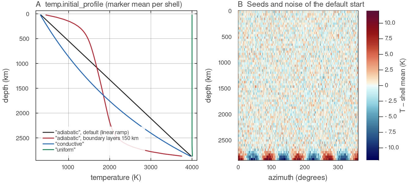
init_markers on the default shell (Nr = 64, Nt = 256), binned per shell. A: the default "adiabatic" choice with zero boundary-layer thickness is the linear ramp; with 150 km thicknesses it becomes the adiabat with exponential boundary layers; "conductive" is the logarithmic profile of the marker initialiser and "uniform" sits at $T_{\text{cmb}}$. B: the default start minus its shell mean, showing the four warm seeds of cfg.m_wavenumber = 4 at the CMB (cfg.dT_anomaly = 20 K, cfg.r_anomaly = 100 km) and the 5 K noise. Script: docs/scripts/fig_heat_sources_sections.jl.

Energy budget

Every row of diagnostics.csv (utils/diagnostics_csv.jl) carries the thermal energy E_th_J $=c_p\sum {\rho }_{\text{ref}}TV$ (thermal_energy), its rate of change dEdt_W since the previous row, the power supplied P_supplied_W (wall power plus internal heating) and budget_resid, the mismatch normalised by the larger of the surface and internal power. The wall power is accumulated every step with the diffusion solver's own $\theta$ weighting (boundary_power), and the internal power from what the solver actually applied (internal_power_last), so the residual tests conservation rather than sampling. Conduction conserves this measure exactly in every mode, since the operator carries $k={\rho }_{\text{ref}}{c}_p\kappa$ inside the divergence (conduction_coefficients). Advection conserves it too, because under ALA and TALA the 2-D Stokes solve enforces $\mathrm{\nabla }\cdot ({\rho }_{\text{ref}}\mathbf{v})=0$ and the grid advection uses the same mass flux,

$$\mathbf{v}\cdot \mathrm{\nabla }T=\frac{1}{{\rho }_{\text{ref}}}[\mathrm{\nabla }\cdot ({\rho }_{\text{ref}}\mathbf{v}T)-T\mathrm{\nabla }\cdot ({\rho }_{\text{ref}}\mathbf{v})],$$

divided by the exact cell measure, so that $\frac{d}{dt}{c}_p\int {\rho }_{\text{ref}}TdV$ changes only by the wall power and the applied sources. With continuity $\mathrm{\nabla }\cdot \mathbf{v}=0$, as before, advection changed it at the rate $c_p\int T{V}_r{\partial }_r{\rho }_{\text{ref}}dV$: on the Earth example with the Perple_X table (density 3349 to 5695 kg m⁻³) that was $-9.3\times {10}^{12}$ W over steps 100 to 200, and budget_resid reached $-0.44$ at step 200 and $-1.29$ at step 300. On the grid-temperature path one full ALA time step now closes to about ${10}^{-12}$ (tests/test_anelastic_mass_balance.jl). On the marker path the hand-back is exact in the mass-weighted measure $\sum _m{\rho }_{\text{ref}}(r_m)w_m{T}_m$ (delivery_scale divides the cell mass by the marker mass of the last projection), but the projection of Lagrangian marker temperatures onto the grid is not conservative, in Boussinesq runs as well, so budget_resid there measures the projection. Under ALA a marker's weight $w_m$ is its current volume: advect_markers! rescales it by ${\rho }_{\text{ref}}(r_{\text{old}})/{\rho }_{\text{ref}}(r_{\text{new}})$ so that its mass is fixed. On the Earth example (marker path, $N_r=64$) budget_resid is now $-0.006$, $-0.015$ and $+0.0005$ at steps 100, 200 and 300; with the anelastic Stokes solve but fixed marker volumes it was $-0.033$ and $-0.31$ at steps 100 and 200, because a parcel carried from the surface into the lower mantle kept the weight of its seeding volume. The 3-D path still solves $\mathrm{\nabla }\cdot \mathbf{v}=0$ under ALA/TALA and its budget_resid contains the $c_p\int T{V}_r{\partial }_r{\rho }_{\text{ref}}dV$ term (validate! warns). In 3-D the wall powers sum the columns of a patch with their own wall areas ($R^2\sin \theta \mathrm{\Delta }\theta \mathrm{\Delta }\phi$, wall_mean), as do the reported $q_{\text{surf}}$, $q_{\text{cmb}}$ and Nusselt numbers. With a cooling core the columns E_core_J, E_cmb_cum_J and budget_resid_joint extend the budget to core plus mantle. In 2-D, marker reseeding is the main operation that is not exactly conservative; it shows in budget_resid. tests/test_marker_energy.jl checks that one marker temperature step hands back exactly the energy the grid solver computed.

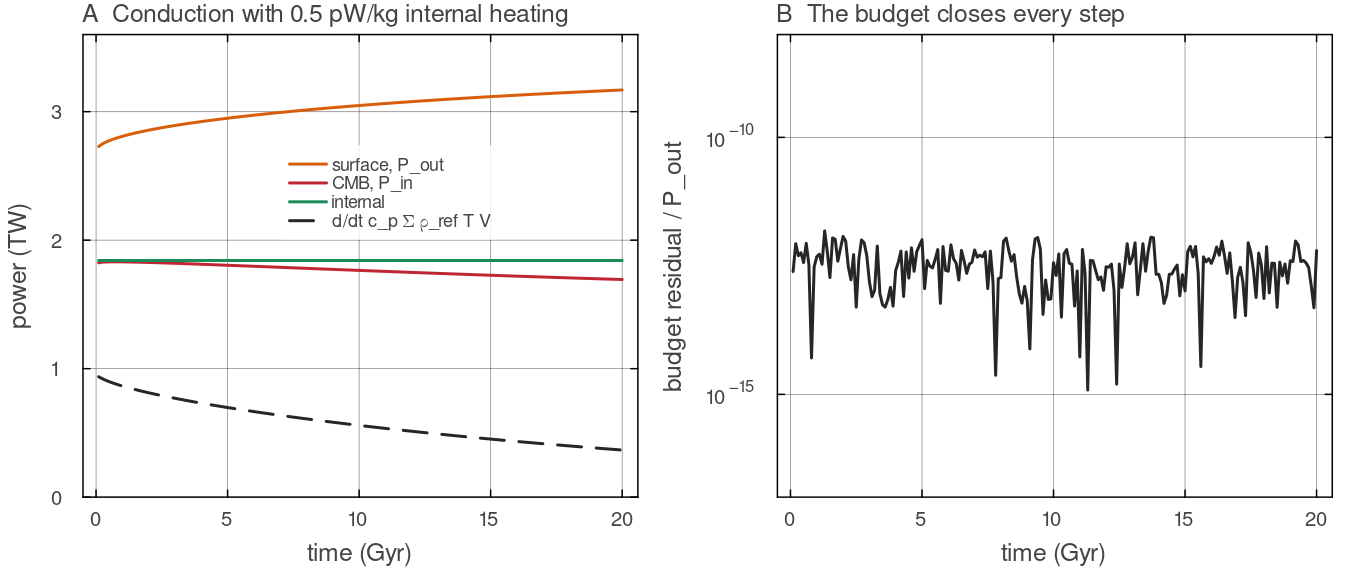
Two hundred backward-Euler steps of 100 Myr of diffuse_temperature in the default shell (Nr = 64, ALA, 0.5 pW kg${}^{-1}$ internal heating) from a linear ramp. A: the wall powers of boundary_power, the internal power of internal_power_last and the change of thermal_energy. B: the residual $|dE/dt-(P_{\text{in}}-P_{\text{out}}+P_{\text{int}})|/P_{\text{out}}$ of every step stays below $2\times {10}^{-12}$. Conduction only; advection and the marker transport, which the paragraphs above discuss, are not part of this test. Script: docs/scripts/fig_heat_sources_sections.jl.

Symbols used on this page

symbol	meaning	unit
$S$	total source added to the conduction term, as a rate of temperature change	K s${}^{-1}$
$H$	heat production per unit mass (radiogenic and uniform internal heating)	W kg${}^{-1}$
$H_0(t)$	planet-wide radiogenic rate after decay, before composition factors	W kg${}^{-1}$
$t_{1/2}$	half-life of the single-rate law (cfg.radioHeatingTau) or of one isotope	yr, Gyr
$c_i$, $h_i$	concentration of isotope chain $i$ and its specific heat production	kg kg${}^{-1}$, W kg${}^{-1}$
$f_{\text{mantle}}$, $f_{\text{cont}}$, $f_{\text{pile}}$	lithology multipliers of the radiogenic rate	1
$f_{\text{dep}}$	heat-producing-element factor of melt depletion	1
$C_{\text{cont}}$, $C_{\text{pile}}$	grid fractions of continental crust and pile material	1
$Q$	volumetric sources and sinks (latent heat, heat pipe, adiabatic term, dissipation)	W m${}^{-3}$
${\rho }_{\text{ref}}$, ${\rho }_0$	reference density profile and constant reference density	kg m${}^{-3}$
$c_p$	specific heat of the mantle, 1250	J kg${}^{-1}$ K${}^{-1}$
$\alpha$, $g$	thermal expansivity and gravitational acceleration	K${}^{-1}$, m s${}^{-2}$
$V_r$	radial velocity, positive outwards	m s${}^{-1}$
$\eta$, ${\dot{\epsilon }}_{II}$	viscosity and second invariant of the strain rate	Pa s, s${}^{-1}$
$L$, $L_k$, $F$, ${\mathrm{\Gamma }}_k$	latent heats, melt fraction and phase function of transition $k$	J kg${}^{-1}$, 1, 1
$\kappa$, $k$	thermal diffusivity and conductivity, $k=\kappa {\rho }_{\text{ref}}{c}_p$	m${}^2$ s${}^{-1}$, W m${}^{-1}$ K${}^{-1}$
$T_{\text{bc}}$, $T_{\text{surf}}$, $T_{\text{cmb}}$	wall temperature, surface temperature, CMB temperature	K
$q_{\text{wall}}$, $Q_{\text{cmb}}$	conductive heat flux through a wall, total heat flow through the CMB	W m${}^{-2}$, W
$C_{\text{core}}$, $V_{\text{core}}$	heat capacity and volume of the core	J K${}^{-1}$, m${}^3$
${\rho }_c$, $c_c$, $f_L$	core density, core specific heat, latent-energy factor	kg m${}^{-3}$, J kg${}^{-1}$ K${}^{-1}$, 1
$\theta$	time-weighting parameter of the temperature solver	1

Assumptions and simplifications

• One specific heat. $c_p=1250$ J kg${}^{-1}$ K${}^{-1}$ everywhere, in mantle, crust and pile alike, so a given power warms every cell of the same density at the same rate.

• Radiogenic heating from a bulk rate. The single-rate law uses one effective half-life. The four-isotope law follows each chain separately but splits uranium and potassium with the modern U-235 and K-40 fractions at $t=0$, so concentrations meant for an early epoch carry the modern isotope ratios. Heat production differs between materials only through the multipliers $f_{\text{mantle}}$, $f_{\text{cont}}$, $f_{\text{pile}}$ and the depletion factor $f_{\text{dep}}$; the 3-D solver applies $f_{\text{dep}}$ alone.

• Fixed surface temperature. temp.T_surf is constant in time. There is no coupling to an evolving atmosphere or climate.

• A simple core. In the parameterised mode the core is a single well-mixed reservoir of sensible heat with no inner core and no internal heat sources; cfg.coreLatentFactor is the only stand-in for latent and gravitational energy. In 2-D the CMB temperature is laterally uniform.

• The $O(Di)$ terms only under ALA. Adiabatic heating and viscous dissipation are carried together under ALA with cfg.useShearHeating = true, and not at all under TALA or Boussinesq, so that the energy balance between them is kept.

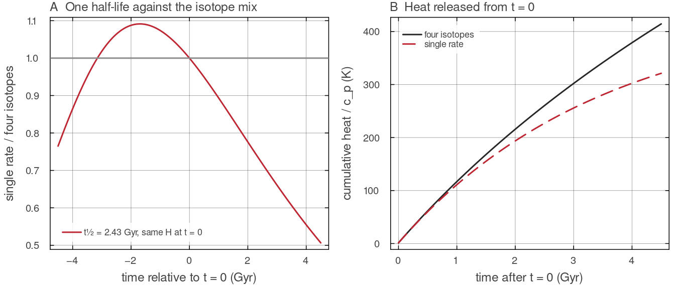
What one effective half-life does. _radiogenic_H0 for the single-rate law ($t_{1/2}$ = 2.43 Gyr, $H_0$ set equal to the four-isotope value at $t=0$) and for the four-isotope law with the default concentrations. A: their ratio lies between 0.76 and 1.09 back to $-4.5$ Gyr, but falls to 0.51 by $+4.5$ Gyr, because the long-lived thorium keeps heating after the effective rate has decayed. B: the heat released from $t=0$, expressed as a temperature rise $\int Hdt/c_p$; after 4.5 Gyr the single rate delivers 321 K against 414 K. The half-life should therefore be chosen for the time window of the run. Script: docs/scripts/fig_heat_sources_sections.jl.

Configuration

field	default	meaning
temp.T_surf, temp.T_cmb	300 K, 4000 K	wall temperatures
cfg.cmbHeatfluxMode	"fixed_T"	fixed_T, fixed_flux or parameterized
cfg.coreDensity, cfg.coreCp, cfg.coreLatentFactor	12 000, 800, 1	core heat capacity
temp.cmb_cooling, temp.cmb_cooling_rate	false, 100 K Gyr${}^{-1}$	prescribed CMB cooling
temp.T_ref	3000 K	floor on an evolving $T_{\text{cmb}}$
cfg.useRadiogenicHeating, cfg.radioHeatingH0, cfg.radioHeatingTau	false, $5\times {10}^{-12}$ W kg${}^{-1}$, 0	single-rate radiogenic heating
cfg.useFourElementRadiogenic	false	isotope-resolved decay
cfg.useInternalHeating, cfg.internalHeating_H	false, 0	uniform internal heating
cfg.useShearHeating	true	adiabatic heating and dissipation under ALA
cfg.useImplicitTemp, cfg.implicitTheta	true, 0.5	time discretisation

Key references

• Stevenson, D. J., Spohn, T. & Schubert, G. (1983). Magnetism and thermal evolution of the terrestrial planets. Icarus 54, 466-489. doi:10.1016/0019-1035(83)90241-5

• Turcotte, D. L. & Schubert, G. (2002). Geodynamics, 2nd ed., Table 4.2. Cambridge University Press. doi:10.1017/CBO9780511807442

• Gerya, T. V. & Yuen, D. A. (2003). Characteristics-based marker-in-cell method with conservative finite-differences schemes for modeling geological flows with strongly variable transport properties. PEPI 140, 293-318. doi:10.1016/j.pepi.2003.09.006

Further reading

• Christensen, U. R. & Yuen, D. A. (1985). Layered convection induced by phase transitions. Journal of Geophysical Research 90, 10291-10300. doi:10.1029/JB090iB12p10291

• Davies, J. H. & Davies, D. R. (2010). Earth's surface heat flux. Solid Earth 1, 5-24. doi:10.5194/se-1-5-2010

• Dziewonski, A. M. & Anderson, D. L. (1981). Preliminary reference Earth model. Physics of the Earth and Planetary Interiors 25, 297-356. doi:10.1016/0031-9201(81)90046-7

• Korenaga, J. (2008). Urey ratio and the structure and evolution of Earth's mantle. Reviews of Geophysics 46, 2007RG000241. doi:10.1029/2007RG000241

• Lay, T., Hernlund, J. & Buffett, B. A. (2008). Core-mantle boundary heat flow. Nature Geoscience 1, 25-32. doi:10.1038/ngeo.2007.44

• Leng, W. & Zhong, S. (2008). Viscous heating, adiabatic heating and energetic consistency in compressible mantle convection. Geophysical Journal International 173, 693-702. doi:10.1111/j.1365-246X.2008.03745.x

• McDonough, W. F. & Sun, S.-s. (1995). The composition of the Earth. Chemical Geology 120, 223-253. doi:10.1016/0009-2541(94)00140-4

• Nimmo, F. (2015). Energetics of the core. In Treatise on Geophysics, 2nd ed., vol. 8, 27-55. Elsevier. doi:10.1016/B978-0-444-53802-4.00139-1

• Nimmo, F. & McKenzie, D. (1998). Volcanism and tectonics on Venus. Annual Review of Earth and Planetary Sciences 26, 23-51. doi:10.1146/annurev.earth.26.1.23

• Rudnick, R. L. & Gao, S. (2003). Composition of the continental crust. In Treatise on Geochemistry, 1-64. Elsevier. doi:10.1016/B0-08-043751-6/03016-4

• Schubert, G., Turcotte, D. L. & Olson, P. (2001). Mantle Convection in the Earth and Planets. Cambridge University Press. doi:10.1017/CBO9780511612879

• Seiff, A., Schofield, J. T., Kliore, A. J., Taylor, F. W. et al. (1985). Models of the structure of the atmosphere of Venus from the surface to 100 kilometers altitude. Advances in Space Research 5, 3-58. doi:10.1016/0273-1177(85)90197-8