Visco-elasto-plasticity

With cfg.useViscoelastoplastic = true the viscosity built by the rheology is passed through viscoelastoplastic (physics/viscoelastoplastic.jl), which combines it with a Maxwell elastic element and a Drucker-Prager stress cap. In MILEVA elasticity acts as a viscosity reduction. The function returns an effective viscosity, and that viscosity is the only part of the calculation that reaches the momentum equation. The deviatoric stress the function also updates is kept between steps but is not fed back into the momentum equation or into the viscosity.

Physical background

Three ways a rock can deform

Rock in a planetary mantle and lithosphere responds to stress in three distinct ways, and which one dominates depends on temperature, pressure, stress and the time scale of loading (Ranalli 1995; Turcotte & Schubert 2014).

• Viscous creep. At high temperature, crystals deform by the slow motion of defects (diffusion and dislocation creep, see flow laws). Stress is proportional to strain rate, and the deformation is permanent. This is the behaviour that lets the mantle convect, with viscosities of order ${10}^{21}$ Pa s inferred for Earth's upper mantle from postglacial rebound (Turcotte & Schubert 2014).

• Elasticity. On short time scales the same rock behaves as a spring. Stress is proportional to strain, with the shear modulus $G$ as the constant, and the strain is recovered when the load is removed. Seismic waves and the flexure of the lithosphere under volcanoes and at trenches are elastic phenomena. The Preliminary Reference Earth Model gives shear moduli of roughly 65 to 80 GPa in the upper 400 km of the mantle (Dziewonski & Anderson 1981).

• Brittle failure and plastic flow. In the cold, near-surface part of the lithosphere, rock fails along faults once the shear stress reaches a strength that grows with confining pressure. Laboratory friction experiments show that this strength depends little on rock type. For normal stress below about 200 MPa the shear stress needed for sliding is about 0.85 times the normal stress, and above it about 50 MPa plus 0.6 times the normal stress (Byerlee 1978). Continuum models represent the many faults of a large region as plastic yielding at a stress limit.

A material that shows all three behaviours is called visco-elasto-plastic. The classical picture of lithospheric strength combines them in a strength envelope. Frictional strength rises with depth near the surface, creep strength falls with depth as temperature rises, and the weaker of the two sets the strength at each depth (Goetze & Evans 1979; Kohlstedt et al. 1995).

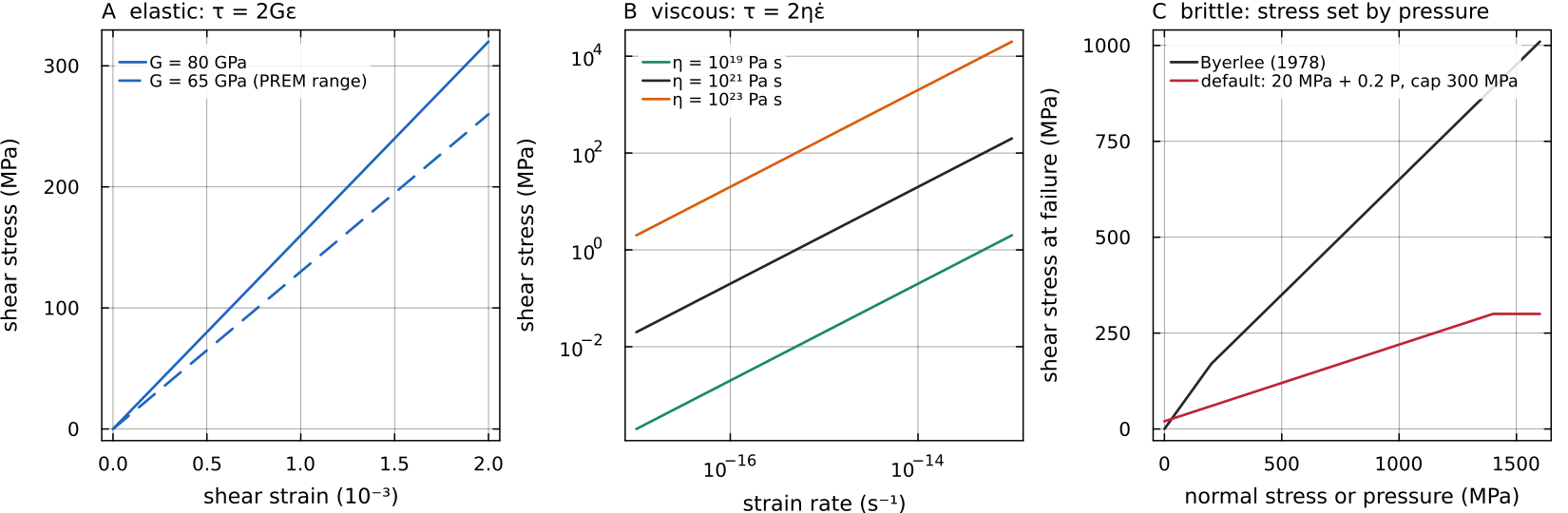
The three responses with the numbers of this section. Left: elasticity, $\tau =2G\epsilon$, for the 65 to 80 GPa of the upper mantle. Middle: viscous creep, $\tau =2\eta \dot{\epsilon }$, for three viscosities; at ${10}^{21}$ Pa s and ${10}^{-15}$ s⁻¹ the stress is 2 MPa. Right: brittle failure, Byerlee's (1978) two-part friction law against the default Drucker-Prager law of viscoelastoplastic (20 MPa + 0.2 P, capped at 300 MPa), which is far weaker. The curves evaluate the elementary laws directly. Script: docs/scripts/fig_viscoelastoplastic_sections.jl.

The Maxwell body and the Maxwell time

The simplest model that is elastic at short times and viscous at long times is the Maxwell body, a spring of modulus $G$ and a dashpot of viscosity $\eta$ in series. Both carry the same stress $\tau$ and their strain rates add,

$$\dot{\epsilon }=\frac{\dot{\tau }}{2G}+\frac{\tau }{2\eta }.$$

Under a constant strain rate the stress builds up as $2\eta \dot{\epsilon }(1-e^{-t/t_M})$, and a stress left on the material decays as $e^{-t/t_M}$, with the Maxwell time

$$t_M=\frac{\eta }{G}.$$

With $G=80$ GPa, $t_M$ is about 4 years for $\eta ={10}^{19}$ Pa s, about 400 years for ${10}^{21}$ Pa s and about 40 kyr for ${10}^{23}$ Pa s. Convecting mantle therefore relaxes elastic stress within centuries and is effectively viscous over the millions of years of convection. A cold lid at ${10}^{24}$ Pa s has a Maxwell time of about 400 kyr, and on the time scale of loading by a volcano or a sinking slab it keeps a memory of elastic stress.

The dimensionless number that compares the two is the Deborah number, the Maxwell time divided by the time scale of the process. In a time-stepping code the natural time scale is the step $\mathrm{\Delta }t$, so

$$\mathrm{De}=\frac{t_M}{\mathrm{\Delta }t}=\frac{\eta }{G\mathrm{\Delta }t}.$$

A Deborah number $\mathrm{De}\ll 1$ means the cell relaxes within one step and behaves viscously; $\mathrm{De}\gg 1$ means it behaves elastically during the step. With the 5 kyr step of the figure below, $G\mathrm{\Delta }t\approx 1.3\times {10}^{22}$ Pa s, so elasticity matters only in cells stiffer than about ${10}^{22}$ Pa s, that is, in the lid.

Left: $t_M=\eta /G$ with $G=80$ GPa, with the values quoted above and the 5 kyr step of the figures below; the Deborah number is 1 where the line crosses the step, at $G\mathrm{\Delta }t\approx 1.3\times {10}^{22}$ Pa s. Right: the Maxwell body of the equation above, analytic, loaded at ${10}^{-15}$ s⁻¹ for 200 kyr and then released. At ${10}^{22}$ Pa s the stress reaches its viscous value $2\eta \dot{\epsilon }$ within about ten kyr and loses it as fast after release; at ${10}^{24}$ Pa s it is still rising when the load stops and keeps most of it 200 kyr later. 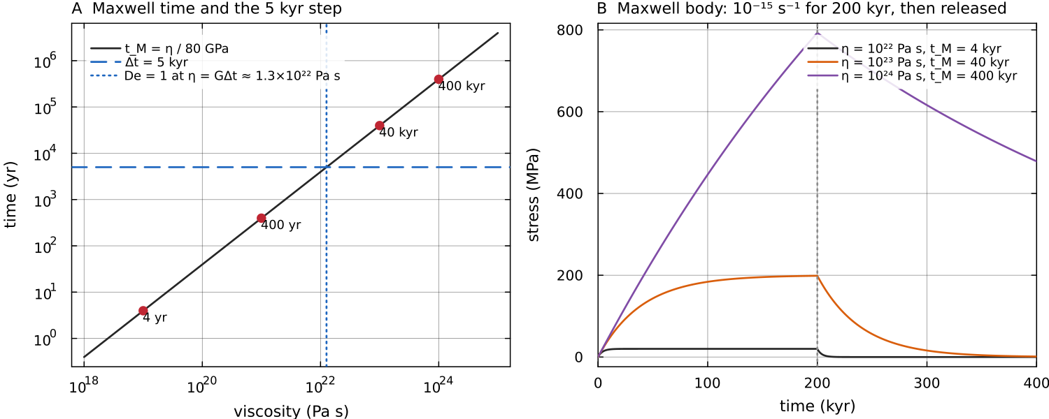Script: docs/scripts/fig_viscoelastoplastic_sections.jl.

Why plasticity matters for planets

Creep viscosity depends exponentially on temperature, so the cold top of a convecting mantle becomes so stiff that it cannot move, and the mantle convects beneath a stagnant lid (Solomatov 1995; see also rheology). A stress limit lets the lid break where convective stresses exceed its strength. Treating that limit as a viscosity cap, $\eta \le {\tau }_y/(2{\dot{\epsilon }}_{II})$, is the pseudo-plastic approach used to obtain plate-like surface motion in convection models (Moresi & Solomatov 1998; Tackley 2000). Moresi & Solomatov (1998) found that plate-like behaviour requires a friction coefficient well below Byerlee's laboratory value, and used the approach to discuss why Earth has mobile plates while Venus, which shows no plate tectonics today, does not. The yield parameters are therefore among the most influential and least constrained choices in a lithosphere model.

Elasticity matters less for the mantle than for the lid. It limits the stress a stiff region can build within one step to about $2G\mathrm{\Delta }t{\dot{\epsilon }}_{II}$, and in formulations that carry the stress history it lets the lithosphere flex and store stress (Moresi et al. 2003; Gerya & Yuen 2007). As the sections below explain, MILEVA keeps the first effect and not the second.

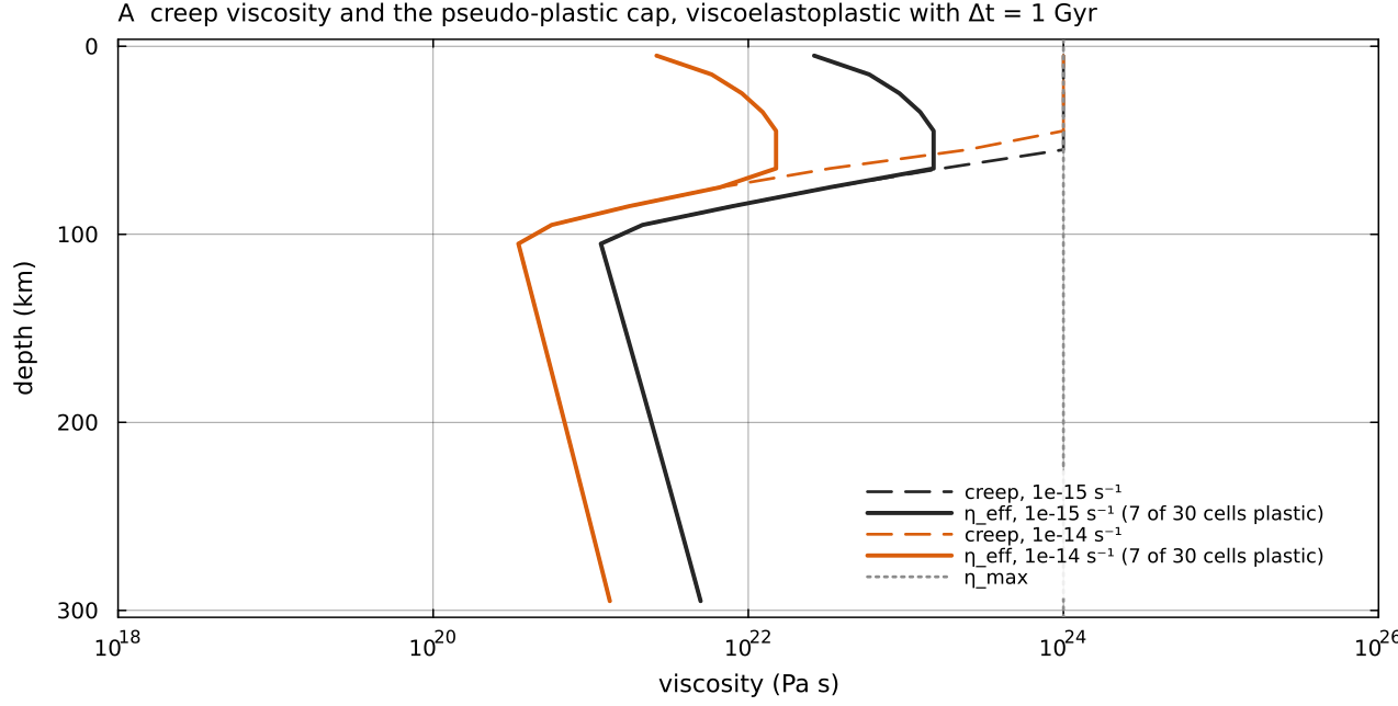
The pseudo-plastic cap on the upper 300 km of a column of 289 cells (10 km each). Dashed: creep viscosity from composite_rheology (yield branch off) on the code's geotherm, which puts the lid at the upper clamp of ${10}^{24}$ Pa s. Solid: the effective viscosity returned by viscoelastoplastic with a step of 1 Gyr, long enough that elasticity plays no part, so only the cap ${\tau }_y/(2{\dot{\epsilon }}_{II})$ acts. It lowers the lid by one to almost three orders of magnitude, more at the higher strain rate, and leaves the mantle below 80 km untouched. Script: docs/scripts/fig_viscoelastoplastic_sections.jl.

The Drucker-Prager criterion

The Drucker-Prager criterion (Drucker & Prager 1952) is a pressure-dependent yield condition on the second invariant of the deviatoric stress. It is a smooth approximation of the Mohr-Coulomb law of faulting and is written as a cohesion plus a friction term that grows with pressure. MILEVA uses the form ${\tau }_y=C+\mu P$, with $\mu$ a friction coefficient in the sense of Byerlee's law and $P$ the lithostatic pressure. With the default ${\rho }_0=3300$ kg m${}^{-3}$ and $g=9.81$ m s${}^{-2}$ the lithostatic pressure grows by about 32 MPa per km, so with $C=20$ MPa and $\mu =0.2$ the yield stress grows by about 6.5 MPa per km and reaches the 300 MPa cap at about 43 km depth. Below that depth the cap, not the pressure, sets the strength.

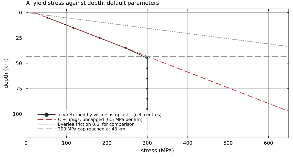
The yield stress as viscoelastoplastic applies it, read from the stress it returns in cells forced to yield (${10}^{-10}$ s⁻¹), at the centres of its uniform 10 km cells. It follows $C+\mu {\rho }_{0}gz$ at 6.5 MPa per km and stays at the 300 MPa cap below 43 km. Byerlee's friction of 0.6 is drawn for comparison. Script: docs/scripts/fig_viscoelastoplastic_sections.jl.

Effective viscosity

The function works cell by cell in a fixed order. It first softens the viscosity with a spring in series (the Maxwell viscosity), uses it to estimate the stress the cell would carry, and compares that stress with the strength of the rock at the cell's depth. A cell whose stress would exceed that strength has its viscosity lowered until the stress equals the strength. The function then advances the stored stress, applies the global viscosity bounds, and hands the viscosity to the Stokes solve.

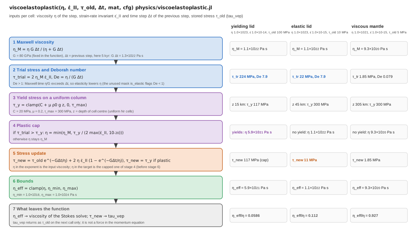
The stages of viscoelastoplastic for three cells of one column of 289 cells with a time step of 5 kyr and the default parameters: a lid cell at 15 km depth ($\eta ={10}^{23}$ Pa s, ${\dot{\epsilon }}_{II}={10}^{-14}$ s${}^{-1}$) yields at 117 MPa and leaves with $5.9\times {10}^{21}$ Pa s; a lid cell at 45 km depth ($\eta ={10}^{23}$ Pa s, ${10}^{-15}$ s${}^{-1}$) stays below its 300 MPa cap and is reduced to the Maxwell value $1.1\times {10}^{22}$ Pa s; a mantle cell at 305 km depth ($\eta ={10}^{21}$ Pa s, ${10}^{-15}$ s${}^{-1}$) keeps $9.3\times {10}^{20}$ Pa s. The values are checked against the function when the figure is made. Script: docs/scripts/fig_viscoelastoplastic_pipeline.jl.

For each cell, with $\eta$ the viscous viscosity of the step (after the creep laws, composition factors and clamps), ${\dot{\epsilon }}_{II}$ the strain-rate invariant of the previous step, $\mathrm{\Delta }t$ the previous time step and a shear modulus $G=80$ GPa fixed in the function:

$${\eta }_M=\frac{\eta G\mathrm{\Delta }t}{\eta +G\mathrm{\Delta }t},{\tau }_{\text{trial}}=2{\eta }_M{\dot{\epsilon }}_{II}.$$

The Maxwell viscosity ${\eta }_M$ tends to $\eta$ when the Maxwell time $\eta /G$ is short compared with $\mathrm{\Delta }t$ (viscous limit) and to $G\mathrm{\Delta }t$ when it is long (elastic limit).

The yield stress is a Drucker-Prager law on a lithostatic pressure,

$${\tau }_y=\mathrm{clamp}(C+\mu {\rho }_{0}gz,0,{\tau }_{\text{max}}),$$

with $C$ = mat.cohesion_upper, $\mu$ = mat.friction_upper and ${\tau }_{\text{max}}$ = mat.maxYieldStress at every depth, and $z$ the depth of the cell centre of a uniform radial grid with the same number of cells. Where ${\tau }_{\text{trial}}>{\tau }_y$ the cell is plastic and

$${\eta }_{\text{eff}}=min({\eta }_M,\frac{{\tau }_y}{2{\dot{\epsilon }}_{II}}),$$

otherwise ${\eta }_{\text{eff}}={\eta }_M$; the strain rate in the denominator is floored at ${10}^{-20}$ s${}^{-1}$. The result is clamped to $[{\eta }_{\text{min}},{\eta }_{\text{max}}]$ and replaces the viscosity for the Stokes solve. The stress update below uses ${\eta }_{\text{eff}}$ before this clamp.

The symbols of this page, with their units and where each value comes from:

symbol	meaning	unit	source in MILEVA
$\eta$	viscous viscosity of the step, before this function	Pa s	ETA from the simple or composite path
${\dot{\epsilon }}_{II}$	second invariant of the strain-rate tensor, $\sqrt{\frac{1}{2}{\dot{\epsilon }}_{ij}{\dot{\epsilon }}_{ij}}$	s${}^{-1}$	strainII of the previous step
$\mathrm{\Delta }t$	time step	s	dt of the previous step
$G$	shear modulus	Pa	80 GPa, fixed in the function
${\eta }_M$	Maxwell (viscoelastic) viscosity	Pa s	computed
${\tau }_{\text{trial}}$	stress the cell would carry at ${\eta }_M$	Pa	computed
$C$, $\mu$	cohesion and friction coefficient	Pa, -	mat.cohesion_upper, mat.friction_upper
${\rho }_0$, $g$, $z$	reference density, gravity, depth of the cell centre	kg m${}^{-3}$, m s${}^{-2}$, m	cfg.rho0, cfg.g, uniform grid
${\tau }_{\text{max}}$	upper limit of the yield stress	Pa	mat.maxYieldStress
${\tau }_y$	yield stress	Pa	computed
${\eta }_{\text{eff}}$	effective viscosity passed to the Stokes solve	Pa s	returned
${\tau }^n$, ${\tau }^{n+1}$	stored scalar stress before and after the step	Pa	tau_vep

Read together, the two equations above make ${\eta }_{\text{eff}}$ (before the global clamp) no larger than the smallest of three viscosities, and close to it when one is much smaller than the others. These are the viscous one $\eta$, the elastic one $G\mathrm{\Delta }t$ (through the series combination, which is always below both), and the plastic one ${\tau }_y/(2{\dot{\epsilon }}_{II})$ where the cell yields. Each of the three cells in the figure illustrates one of these limits.

Stress update

The function also advances a scalar stress per cell, held by the driver in the grid array tau_vep (zero at the start of the run):

$${\tau }^{n+1}={\tau }^n{e}^{-G\mathrm{\Delta }t/\eta }+2{\eta }_{\text{eff}}{\dot{\epsilon }}_{II}(1-e^{-G\mathrm{\Delta }t/\eta }),{\tau }^{n+1}={\tau }_y\text{in plastic cells}.$$

Under a constant strain rate this relaxes toward $2{\eta }_{\text{eff}}{\dot{\epsilon }}_{II}$ with the Maxwell time $\eta /G$. In the elastic limit that target is $2G\mathrm{\Delta }t{\dot{\epsilon }}_{II}$, so the stress the function records depends on the time step and does not approach the viscous stress $2\eta {\dot{\epsilon }}_{II}$ (left panel of the figure).

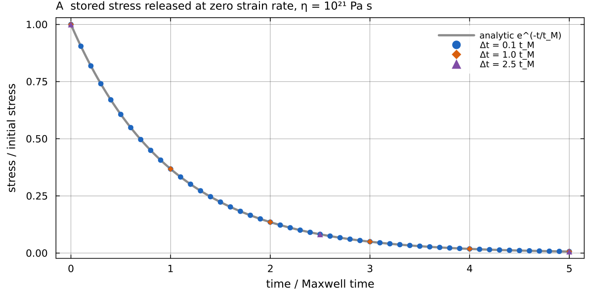
A stress of 2 MPa stored in a column at ${10}^{21}$ Pa s, released by calling viscoelastoplastic repeatedly with zero strain rate and time steps of 0.1, 1 and 2.5 Maxwell times. The update multiplies by $e^{-G\mathrm{\Delta }t/\eta }$, so the relaxation of stored stress is exact at any step; only the build-up term depends on the step, as the figure in the next section shows. Script: docs/scripts/fig_viscoelastoplastic_sections.jl.

What enters the momentum equation

quantity	used by the Stokes solve
${\eta }_{\text{eff}}$	yes, as the viscosity of the step
${\tau }^{n+1}$ (tau_vep)	no; it is passed back as ${\tau }^n$ on the next call and used only in the stress update itself
elastic mask (Deborah number $\eta /G\mathrm{\Delta }t>1$) and plastic mask	no; returned and not used by the driver. The elastic mask marks the cells whose Maxwell time is longer than the step, the elastic ones in the sense of the Deborah number above

There is no elastic stress-history term on the right-hand side of the momentum equation, so material does not recover elastic strain. tau_vep is a cell field, not a marker field. It stays at its grid position, is not advected, and is not written to checkpoints or VTK output.

In the time loop. viscoelastoplastic is called in step 2 of main_SphCon.jl, after the simple or composite viscosity and before damage, when $\mathrm{\Delta }t>0$ (so not on the first step). On the composite path the nonlinear iteration rebuilds the viscosity with composite_rheology in every sweep after the first and reapplies only the damage factor, so the solve that ends a multi-sweep iteration uses the viscosity without the Maxwell and plastic reduction of this page. The composite path has its own Drucker-Prager branch with strain weakening; the cap here is a second, independent one with the upper-mantle parameters and no temperature gate.

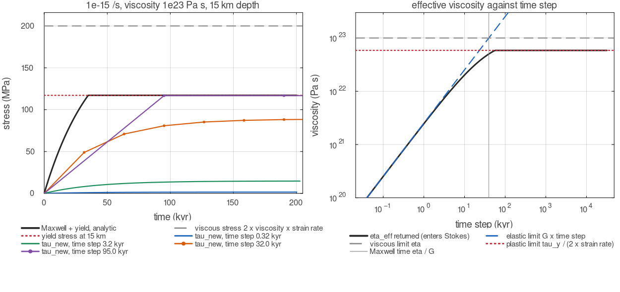
viscoelastoplastic called repeatedly on a column of 290 cells at constant strain rate ${10}^{-15}$ s${}^{-1}$ and viscosity ${10}^{23}$ Pa s, read at the cell centred at 15 km depth (yield stress 117 MPa with the default cohesion and friction). Left: the stress tau_new for four time steps, against the analytic Maxwell build-up $2\eta \dot{\epsilon }(1-e^{-Gt/\eta })$ capped at the yield stress. Right: the effective viscosity the function returns after one call, against the time step, with the elastic ($G\mathrm{\Delta }t$), viscous ($\eta$) and plastic (${\tau }_y/2\dot{\epsilon }$) limits.

Assumptions and simplifications

The function is a deliberately reduced form of visco-elasto-plasticity. Each simplification below follows from the code and has a reason.

• Elasticity as a viscosity reduction only. A full viscoelastic formulation evaluates the trial stress as $2{\eta }_M{\dot{\epsilon }}_{II}$ plus a term proportional to the stress of the previous step, and adds the advected old stress to the right-hand side of the momentum equation (Moresi et al. 2003; Gerya & Yuen 2007). MILEVA's trial stress is $2{\eta }_M{\dot{\epsilon }}_{II}$ alone, and the momentum equation contains no stress-history term. The model therefore captures the time-step-limited stress of stiff cells but not elastic flexure or the recovery of elastic strain. For mantle convection over millions of years this is the regime that matters most: at ${10}^{21}$ Pa s and a 10 kyr step, $\mathrm{De}=0.04$, so a mantle of that viscosity relaxes within a step. Cells stiffer than $G\mathrm{\Delta }t$, about $2.5\times {10}^{22}$ Pa s at 10 kyr, have $\mathrm{De}>1$; the figure below shows where that happens with the default creep laws.

• A scalar, Eulerian stress. tau_vep is one number per cell rather than a stress tensor, and it is not carried with the material. This is consistent with its role, since it does not reach the momentum equation.

• Lithostatic pressure in the yield law. The pressure is ${\rho }_{0}gz$ on a uniform radial grid, not the dynamic pressure of the Stokes solution and not the pressure on a stretched grid. This keeps the yield stress a fixed, smooth function of depth that cannot feed back on the flow through the pressure.

• One set of yield parameters. Cohesion and friction are the upper-mantle values at every depth and in every material, with no temperature gate and no strain weakening. In practice the 300 MPa cap sets the strength below about 43 km with the defaults. In convecting mantle the stress is far below any of these values. At ${10}^{21}$ Pa s and ${10}^{-15}$ s${}^{-1}$ it is 2 MPa, so the cap acts only in the lid.

• A constant shear modulus. $G=80$ GPa is a representative upper-mantle value. It enters only through $G\mathrm{\Delta }t$ and the relaxation factor, and matters only in cells with $\mathrm{De}$ near or above one.

• Lagged strain rate. ${\dot{\epsilon }}_{II}$ and $\mathrm{\Delta }t$ are those of the previous step, so the viscosity cap is explicit in time.

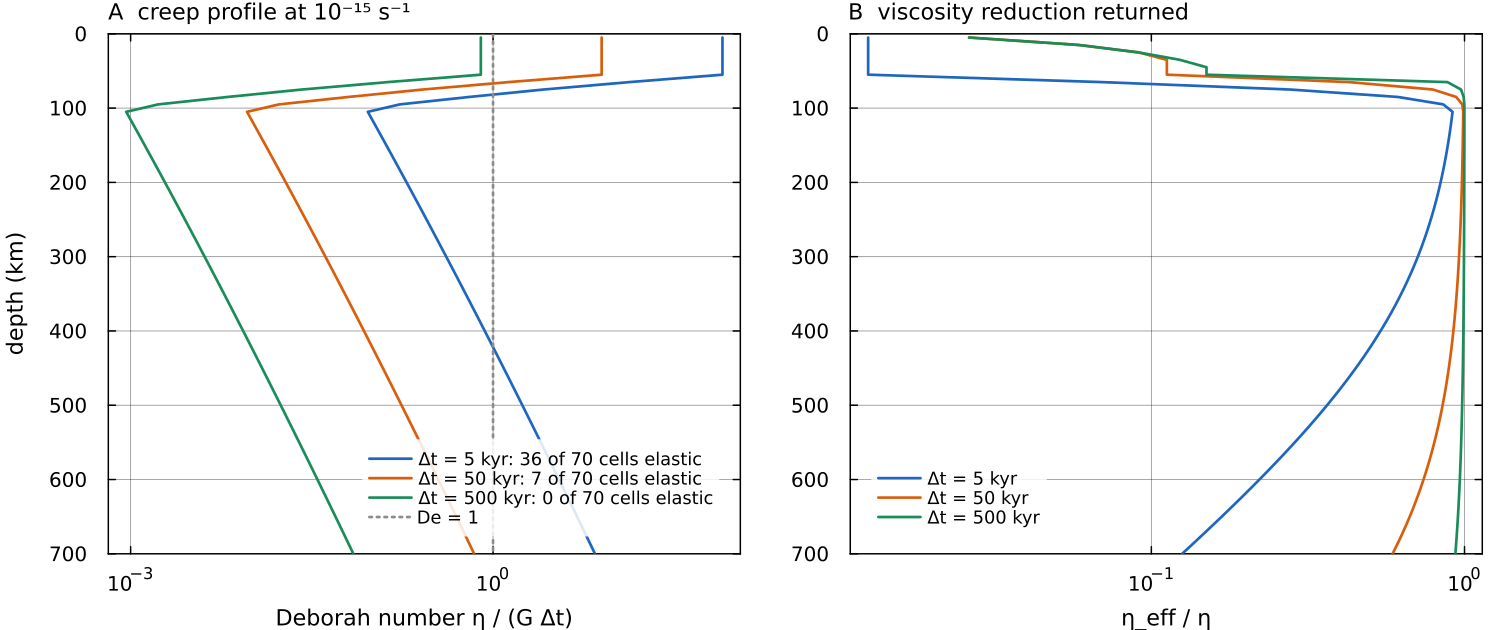
Where the elastic reduction acts. Left: the Deborah number $\eta /(G\mathrm{\Delta }t)$ of the creep profile of composite_rheology (yield off, default clamps, ${10}^{-15}$ s⁻¹) in the upper 700 km, for steps of 5, 50 and 500 kyr, with the number of cells viscoelastoplastic marks as elastic. Right: the ratio ${\eta }_{\text{eff}}/\eta$ it returns. With the default creep laws the viscosity grows with depth, so at a 5 kyr step about half of these cells have $\mathrm{De}>1$; a longer step or a less viscous mantle confines the effect to the lid, where the cap also acts. Script: docs/scripts/fig_viscoelastoplastic_sections.jl.

Scope

The page describes an optional reduction of the viscosity, off by default. It is not a substitute for a viscoelastic formulation with stress advection when elastic flexure or stress transfer is the subject of a study.

2-D and 3-D

The function accepts 2-D and 3-D cell arrays; the pressure column is broadcast over $\theta$ in the annulus and over $(\theta ,\varphi )$ on the Yin-Yang patch. The physics is the same in both.

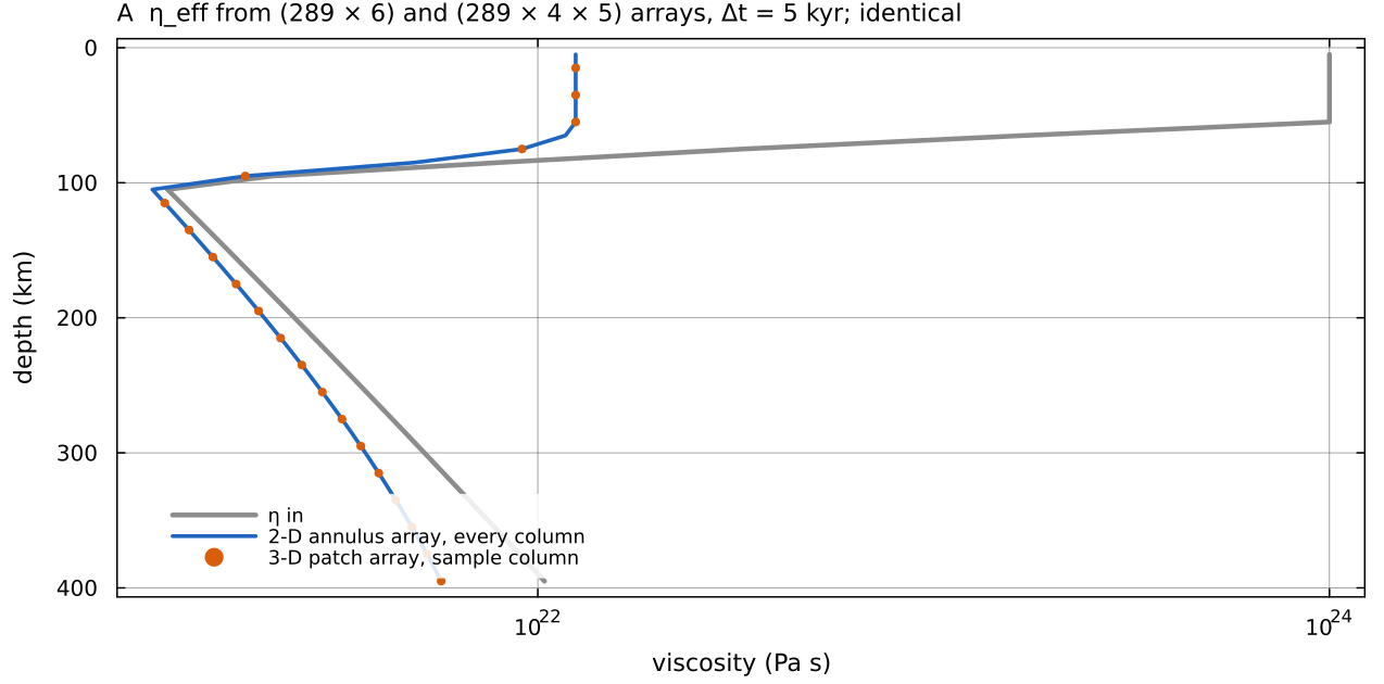
The same column (creep viscosity of the figure above, ${10}^{-15}$ s⁻¹, 5 kyr) passed to viscoelastoplastic as a $289\times 6$ annulus array and as a $289\times 4\times 5$ Yin-Yang patch array. Every column of both returns the same effective viscosity, bit for bit. Script: docs/scripts/fig_viscoelastoplastic_sections.jl.

Configuration

field	default	meaning
cfg.useViscoelastoplastic	false	apply the Maxwell and plastic reduction
mat.cohesion_upper	20 MPa	cohesion $C$
mat.friction_upper	0.2	friction coefficient $\mu$
mat.maxYieldStress	300 MPa	cap ${\tau }_{\text{max}}$
cfg.eta_min, cfg.eta_max	${10}^{18}$, ${10}^{24}$ Pa s	clamps on ${\eta }_{\text{eff}}$
cfg.rho0, cfg.g	3300 kg m${}^{-3}$, 9.81 m s${}^{-2}$	lithostatic pressure of the cap

The shear modulus (80 GPa) is fixed in the function.

Where in the code

What	File, function
Maxwell viscosity, cap, stress update	physics/viscoelastoplastic.jl: viscoelastoplastic
call, tau_vep storage	main_SphCon.jl, step 2
the composite path's own yield branch	physics/composite_rheology.jl: composite_rheology

Tests

• tests/test_config_matrix.jl: visco-elasto-plasticity is off by default.

Key references

• Moresi, L., Dufour, F. & Mühlhaus, H.-B. (2003). A Lagrangian integration point finite element method for large deformation modeling of viscoelastic geomaterials. J. Comput. Phys. 184, 476-497. doi:10.1016/S0021-9991(02)00031-1

• Gerya, T. V. & Yuen, D. A. (2007). Robust characteristics method for modelling multiphase visco-elasto-plastic thermo-mechanical problems. PEPI 163, 83-105. doi:10.1016/j.pepi.2007.04.015

• Drucker, D. C. & Prager, W. (1952). Soil mechanics and plastic analysis or limit design. Q. Appl. Math. 10, 157-165. doi:10.1090/qam/48291

Further reading

• Byerlee, J. (1978). Friction of rocks. Pure Appl. Geophys. 116, 615-626. doi:10.1007/BF00876528

• Dziewonski, A. M. & Anderson, D. L. (1981). Preliminary reference Earth model. Phys. Earth Planet. Inter. 25, 297-356. doi:10.1016/0031-9201(81)90046-7

• Gerya, T. (2019). Introduction to Numerical Geodynamic Modelling, 2nd ed. Cambridge University Press. doi:10.1017/9781316534243

• Goetze, C. & Evans, B. (1979). Stress and temperature in the bending lithosphere as constrained by experimental rock mechanics. Geophys. J. Int. 59, 463-478. doi:10.1111/j.1365-246X.1979.tb02567.x

• Kohlstedt, D. L., Evans, B. & Mackwell, S. J. (1995). Strength of the lithosphere: constraints imposed by laboratory experiments. J. Geophys. Res. 100, 17587-17602. doi:10.1029/95JB01460

• Moresi, L. & Solomatov, V. (1998). Mantle convection with a brittle lithosphere: thoughts on the global tectonic styles of the Earth and Venus. Geophys. J. Int. 133, 669-682. doi:10.1046/j.1365-246X.1998.00521.x

• Ranalli, G. (1995). Rheology of the Earth, 2nd ed. Chapman & Hall.

• Solomatov, V. S. (1995). Scaling of temperature- and stress-dependent viscosity convection. Phys. Fluids 7, 266-274. doi:10.1063/1.868624

• Tackley, P. J. (2000). Self-consistent generation of tectonic plates in time-dependent, three-dimensional mantle convection simulations. Geochem. Geophys. Geosyst. 1. doi:10.1029/2000GC000036

• Turcotte, D. L. & Schubert, G. (2014). Geodynamics, 3rd ed. Cambridge University Press. doi:10.1017/CBO9780511843877